Introduction

Introduction to Statistical Learning - PISE

Aldo Solari

Ca’ Foscari University of Venice

Statistical Learning Problems

• Predicting future values

• Recommender Systems

• Dimension Reduction

• …

Predicting future values

Predicting the food delivery time

• Machine learning models are mathematical equations that take inputs, called predictors, and try to estimate some future output value, called outcome.

\underset{outcome}{Y} \leftarrow f(\underset{predictors}{X_1,\ldots,X_p})

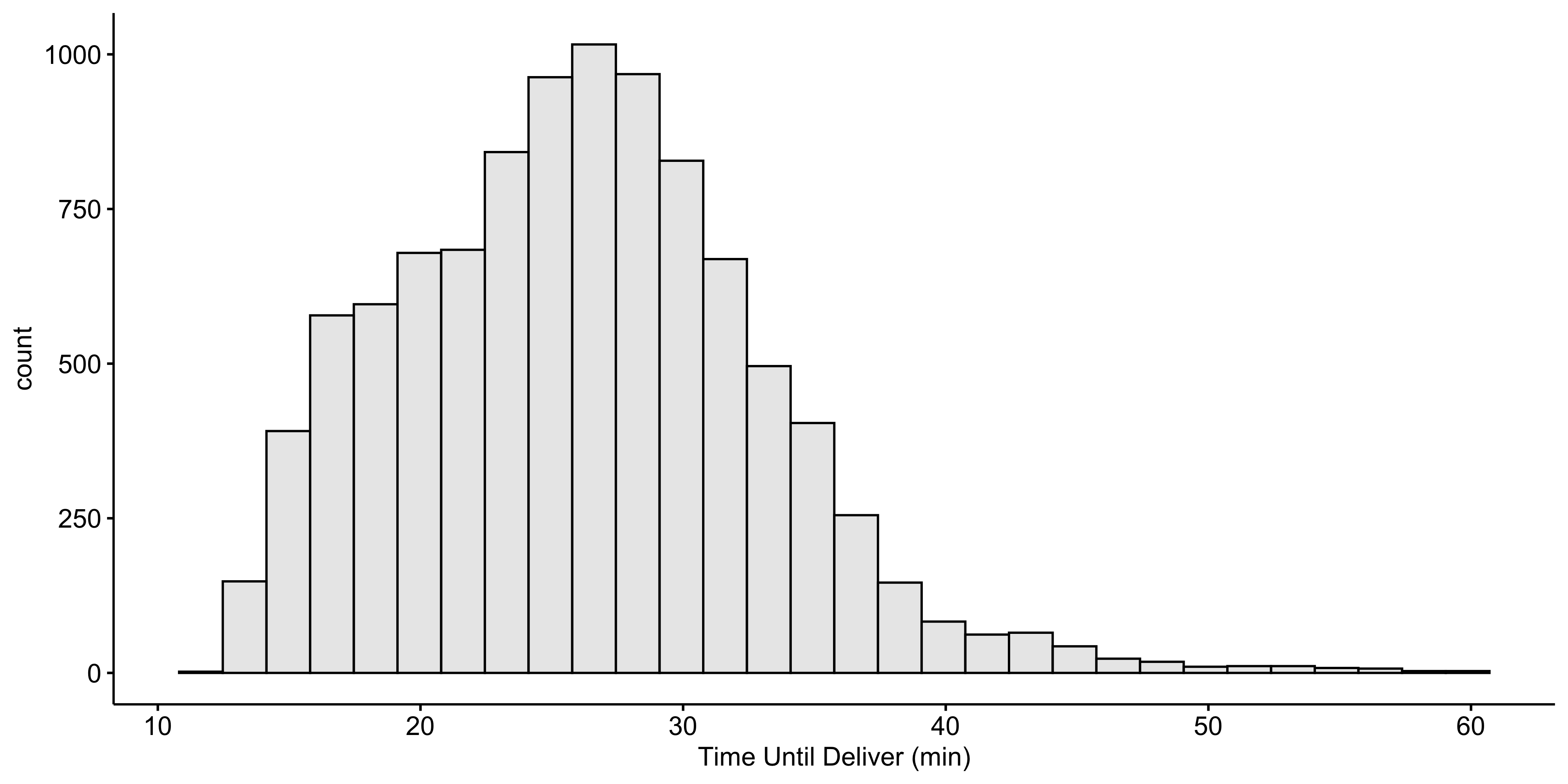
• For example, we want to predict how long it takes to deliver food ordered from a restaurant.

• The outcome is the time from the initial order (in minutes).

• There are multiple predictors, including:

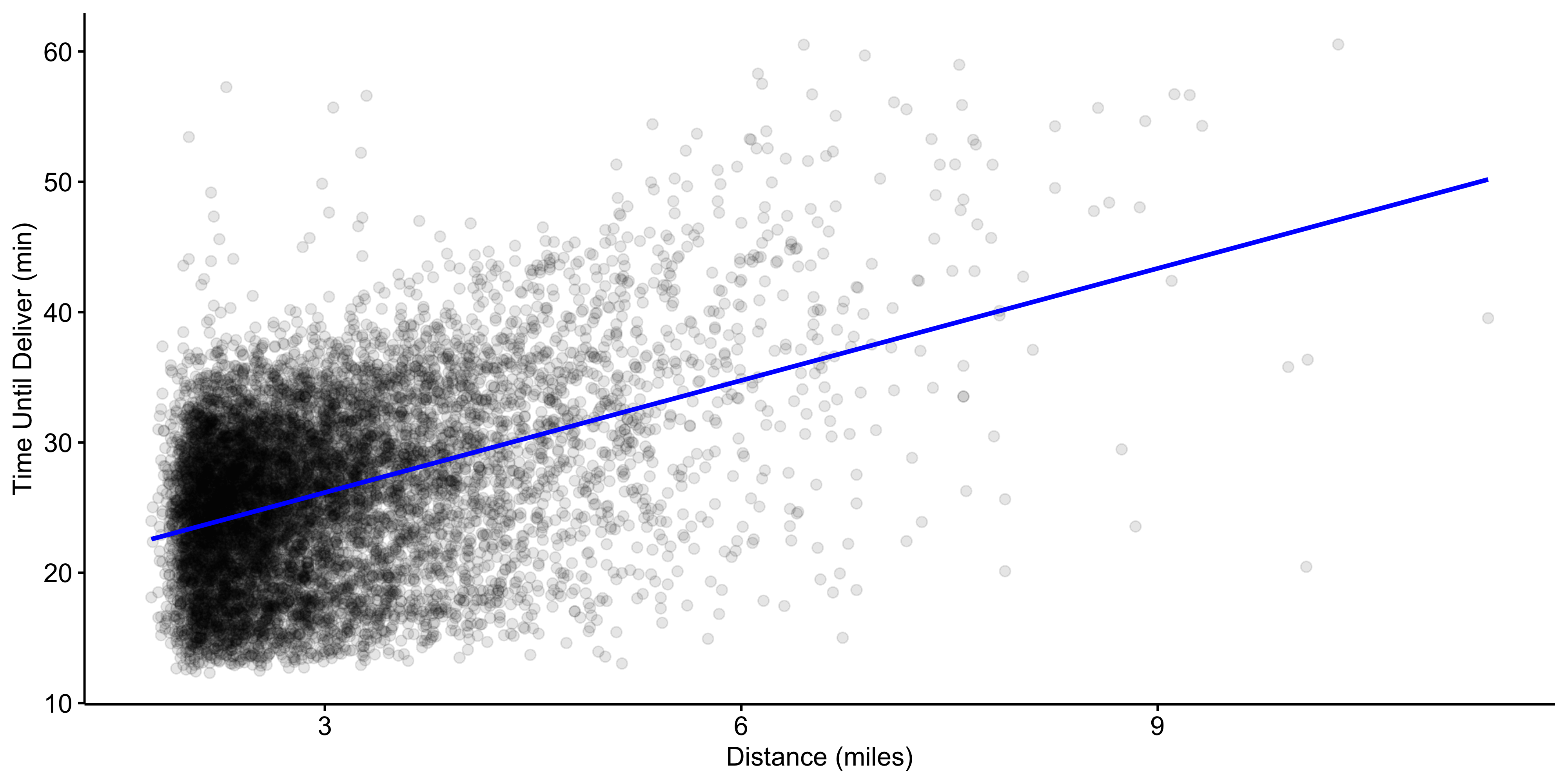
  • the distance from the restaurant to the delivery location,
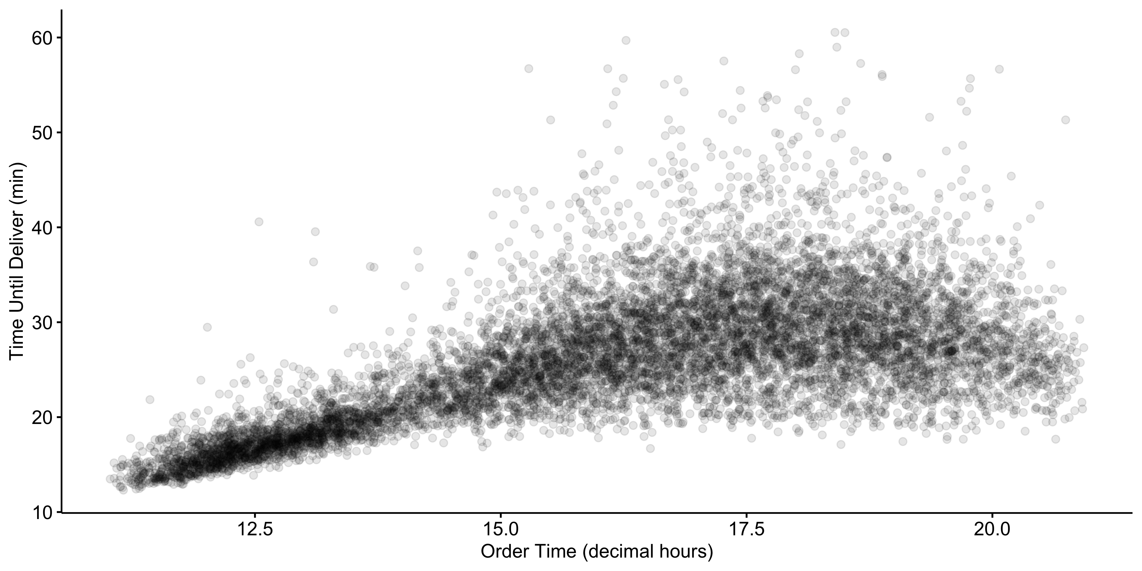
  • the date/time of the order,
  • which items were included in the order.

Food Delivery Time Data

• The data are tabular, where the 31 variables (1 outcome + 30 predictors) are arranged in columns and the the n=10012 observations in rows:

  time_to_delivery   hour day distance item_01 item_02 item_03 item_04 item_27
1          16.1106 11.899 Thu 5.069421       0       0       2       0       0
2          22.9466 19.230 Tue 5.938465       0       0       0       0       0
3          30.2882 18.374 Fri 3.315240       0       0       0       0       0
4          33.4266 15.836 Thu 9.607760       0       0       0       0       1
5          27.2255 19.619 Fri 4.055537       0       0       0       1       1
6          19.6459 12.952 Sat 5.391289       1       0       0       1       0

• Note that the predictor values are known. For future data, the outcome is unknown; it is a machine learning model’s job to predict unknown outcome values.

Outcome Y

Predictor X_1

Regression function

• A machine learning model has a defined mathematical prediction equation, called regression function f(\cdot), defining exactly how the predictors X_1,\ldots,X_n relate to the outcome Y: Y \approx f(X_1,\ldots,X_p)

• Here is a simple example of regression function: the linear model with a single predictor (the distance X_1) and two unknown parameters \beta_0 and \beta_1 that have been estimated:

\begin{aligned} Y &\approx \hat{\beta}_0 + \hat{\beta}_1 X_1\\ \\ delivery\,\,time &\approx 17.557 + 1.781\,\times \,distance \end{aligned}

• We could use this equation for new orders:

  • If we had placed an order at the restaurant (i.e., a zero distance) we predict that it would take 17.5 minutes.

  • If we were seven kilometers away, the predicted delivery time is 17.557 + 7\times 1.781 \approx 30 minutes.

Predictor X_2

3D scatter plot

Regression plane

With two predictors, say X_1 and X_2, the linear regression function becomes a plane in the three-dimensional space: Y \approx \hat\beta_0 + \hat\beta_1 X_1 + \hat\beta_2 X_2.

The fitted regression function is delivery\,\,time \approx −11.17 + 1.76 \times distance + 1.77 \times order\,\,time

If an order were placed at 12:00 with a distance of 7 km, the predicted delivery time would be −11.17 + 1.76 \times 7 + 1.77 \times 12 = 22.4 minutes.

Regression spline (non-parametric)

Flexibility versus Interpretability

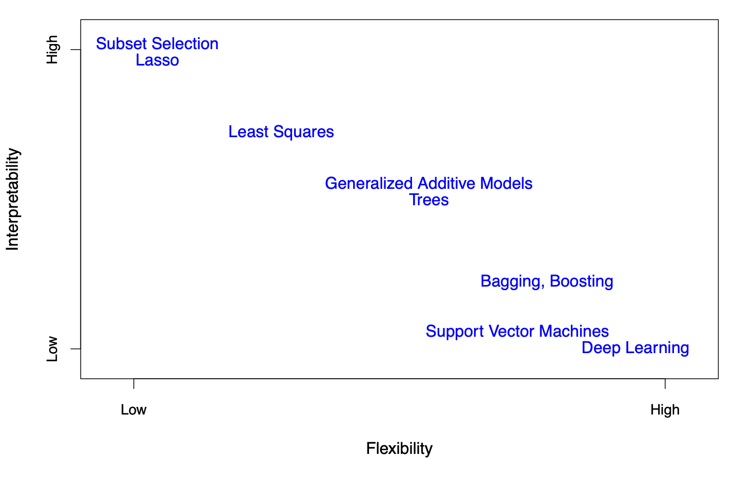
Figure 2.7 (ISL). Representation of the tradeoff between flexibility and interpretability across statistical learning methods. In general, as flexibility increases, interpretability decreases.

Regression tree

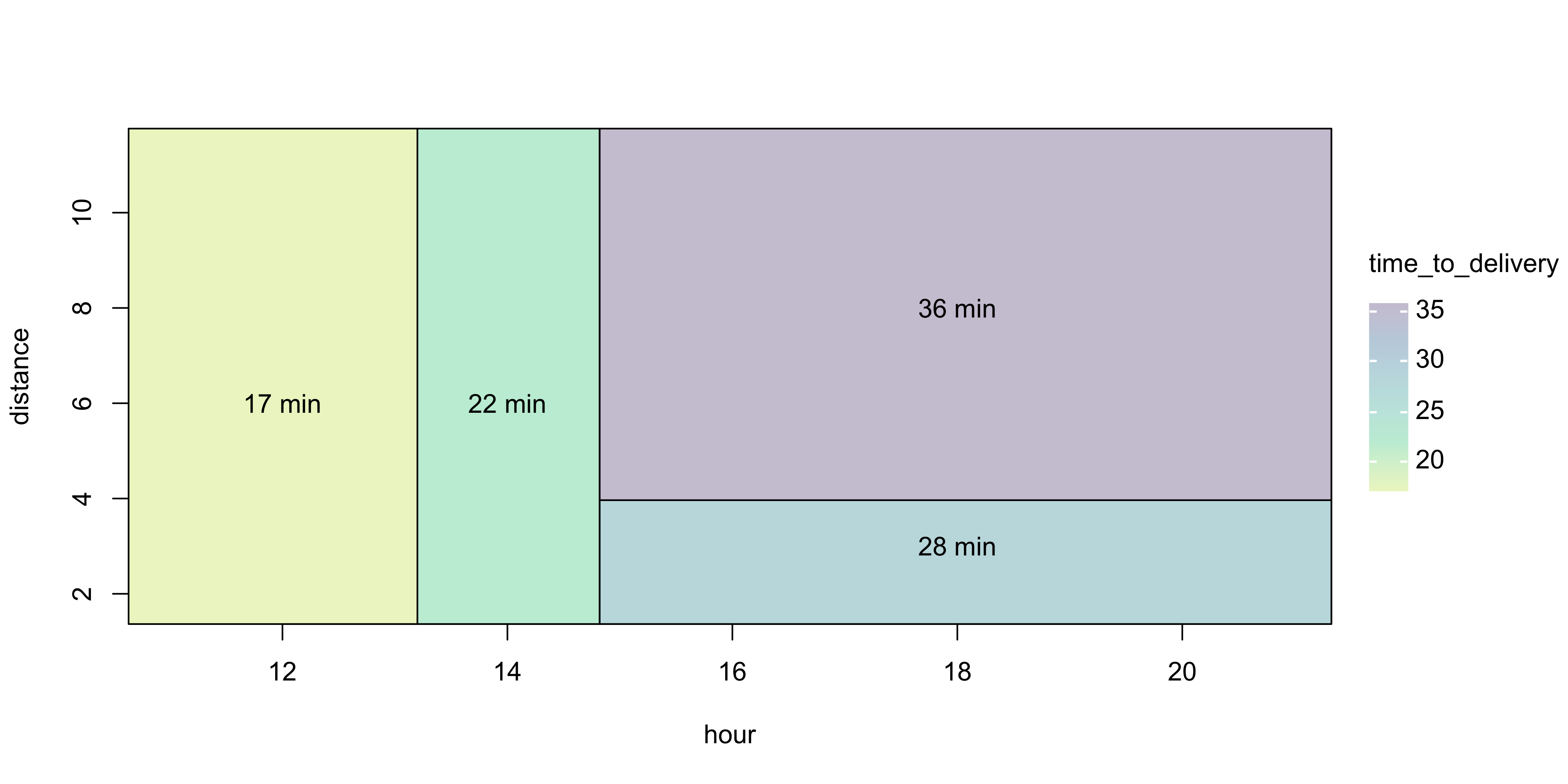
A different regression function

\begin{align} delivery \,\, time \approx \:&17\times\, I\left(\,order\,\,time < 13 \text{ hours } \right) + \notag \\ \:&22\times\, I\left(\,13\leq \, order\,\,time < 15 \text{ hours } \right) + \notag \\ \:&28\times\, I\left(\,order\,\,time \geq 15 \text{ hours and }distance < 6.4 \text{ kilometers }\right) + \notag \\ \:&36\times\, I\left(\,order\,\,time \geq 15 \text{ hours and }distance \geq 6.4 \text{ kilometers }\right)\notag \end{align}

• The indicator function I(\cdot) is one if the logical statement is true and zero otherwise.

• Two predictors (distance X_1 and order time X_2) were used in this case.

Partition of the predictors space (X_1,X_2)

Predictor X_3

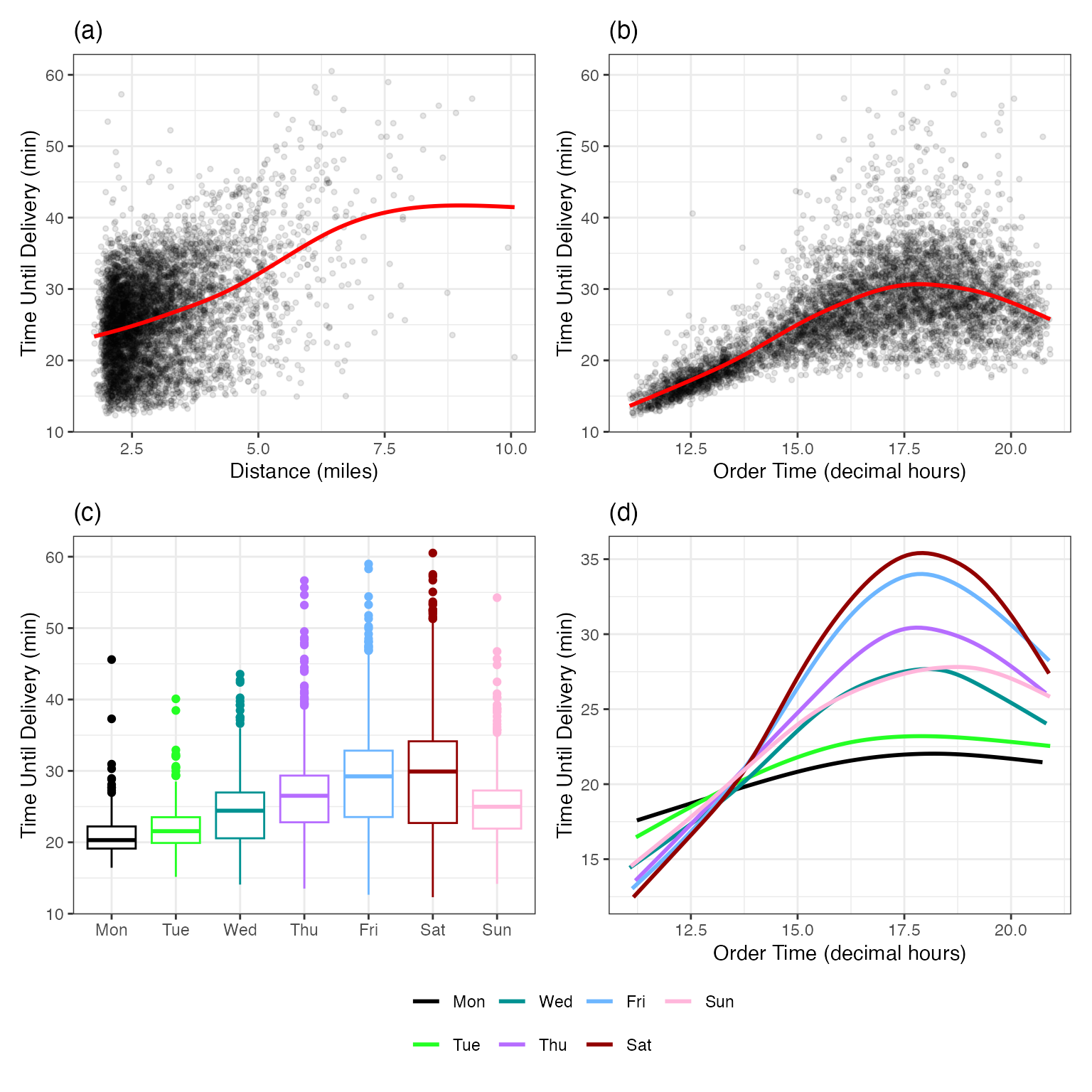
Figure 2.2 in Kuhn, M and Johnson, K (2023) Applied Machine Learning for Tabular Data. https://aml4td.org/

Recommender Systems

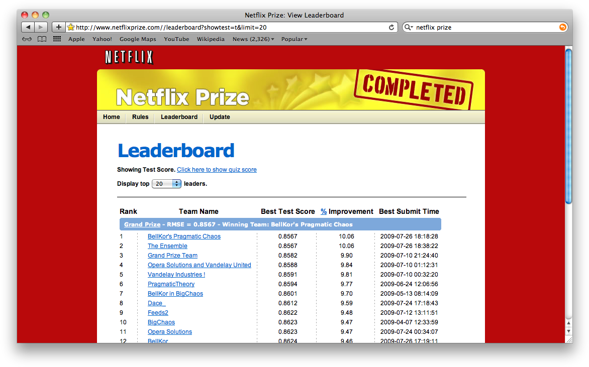
The Netflix Prize

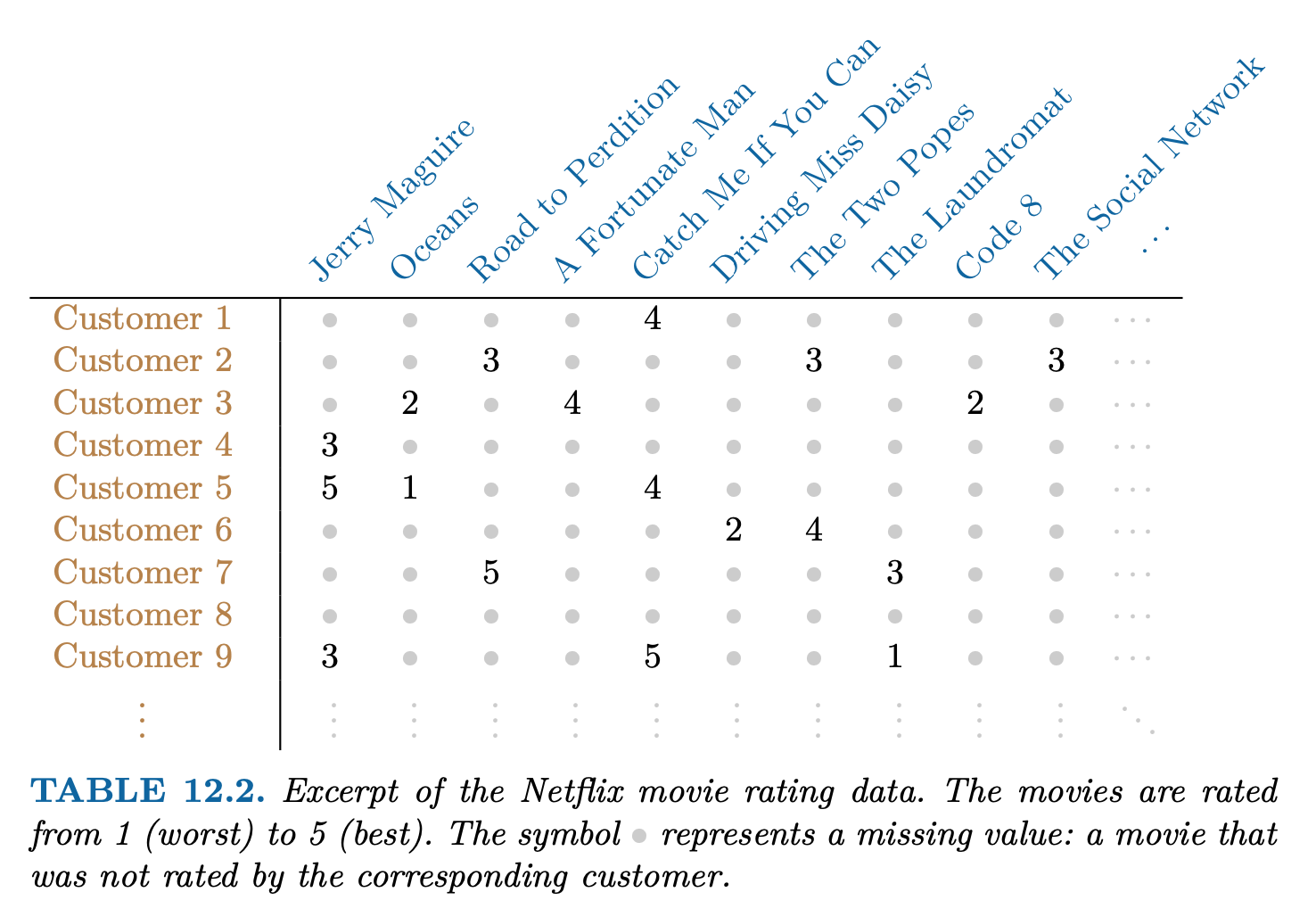
• Competition started in October 2006. The data is ratings for 18000 movies by 400000 Netflix customers, each rating between 1 and 5.

• Data is very sparse - about 98% missing.

• Objective is to predict the rating for a set of 1 million customer-movie pairs that are missing in the data.

• Netflix’s original algorithm achieved a Root Mean Squared Error (RMSE) of 0.953. The first team to achieve a 10% improvement wins one million dollars.

Recommender Systems

• Digital streaming services like Netflix and Amazon use data about the content that a customer has viewed in the past, as well as data from other customers, to suggest other content for the customer.

• In order to suggest a movie that a particular customer might like, Netflix needed a way to impute the missing values of the customer-movie data matrix.

• Principal Component Analysis (PCA) is at the heart of many recommender systems. Principal components can be used to impute the missing values, through a process known as matrix completion.

Dimension Reduction

Heptathlon data

• 100m hurdles.

• high jump.

• shot.

• 200m race.

• long jump.

• javelin.

• 800m race.

Results in the women’s heptathlon in the 1988 Olympics held in Seoul are given in the next table (timed events have times in seconds, distances are measured in metres).

	hurdles	highjump	shot	run200m	longjump	javelin	run800m	score
Joyner-Kersee (USA)	12.69	1.86	15.80	22.56	7.27	45.66	128.51	7291
John (GDR)	12.85	1.80	16.23	23.65	6.71	42.56	126.12	6897
Behmer (GDR)	13.20	1.83	14.20	23.10	6.68	44.54	124.20	6858
Sablovskaite (URS)	13.61	1.80	15.23	23.92	6.25	42.78	132.24	6540
Choubenkova (URS)	13.51	1.74	14.76	23.93	6.32	47.46	127.90	6540
Schulz (GDR)	13.75	1.83	13.50	24.65	6.33	42.82	125.79	6411
Fleming (AUS)	13.38	1.80	12.88	23.59	6.37	40.28	132.54	6351
Greiner (USA)	13.55	1.80	14.13	24.48	6.47	38.00	133.65	6297
Lajbnerova (CZE)	13.63	1.83	14.28	24.86	6.11	42.20	136.05	6252
Bouraga (URS)	13.25	1.77	12.62	23.59	6.28	39.06	134.74	6252
Wijnsma (HOL)	13.75	1.86	13.01	25.03	6.34	37.86	131.49	6205
Dimitrova (BUL)	13.24	1.80	12.88	23.59	6.37	40.28	132.54	6171
Scheider (SWI)	13.85	1.86	11.58	24.87	6.05	47.50	134.93	6137
Braun (FRG)	13.71	1.83	13.16	24.78	6.12	44.58	142.82	6109
Ruotsalainen (FIN)	13.79	1.80	12.32	24.61	6.08	45.44	137.06	6101
Yuping (CHN)	13.93	1.86	14.21	25.00	6.40	38.60	146.67	6087
Hagger (GB)	13.47	1.80	12.75	25.47	6.34	35.76	138.48	5975
Brown (USA)	14.07	1.83	12.69	24.83	6.13	44.34	146.43	5972
Mulliner (GB)	14.39	1.71	12.68	24.92	6.10	37.76	138.02	5746
Hautenauve (BEL)	14.04	1.77	11.81	25.61	5.99	35.68	133.90	5734
Kytola (FIN)	14.31	1.77	11.66	25.69	5.75	39.48	133.35	5686
Geremias (BRA)	14.23	1.71	12.95	25.50	5.50	39.64	144.02	5508
Hui-Ing (TAI)	14.85	1.68	10.00	25.23	5.47	39.14	137.30	5290
Jeong-Mi (KOR)	14.53	1.71	10.83	26.61	5.50	39.26	139.17	5289
Launa (PNG)	16.42	1.50	11.78	26.16	4.88	46.38	163.43	4566

Goal

Determine a score to assign to each athlete that summarizes the performances across the seven events in order to obtain the final ranking, that is, to reduce the dimensionality from 7 to 1.

\underset{25 \times 7}{X} \mapsto \color{red}{\underset{25 \times 1}{y}}

\underset{243 \times 220}{X}

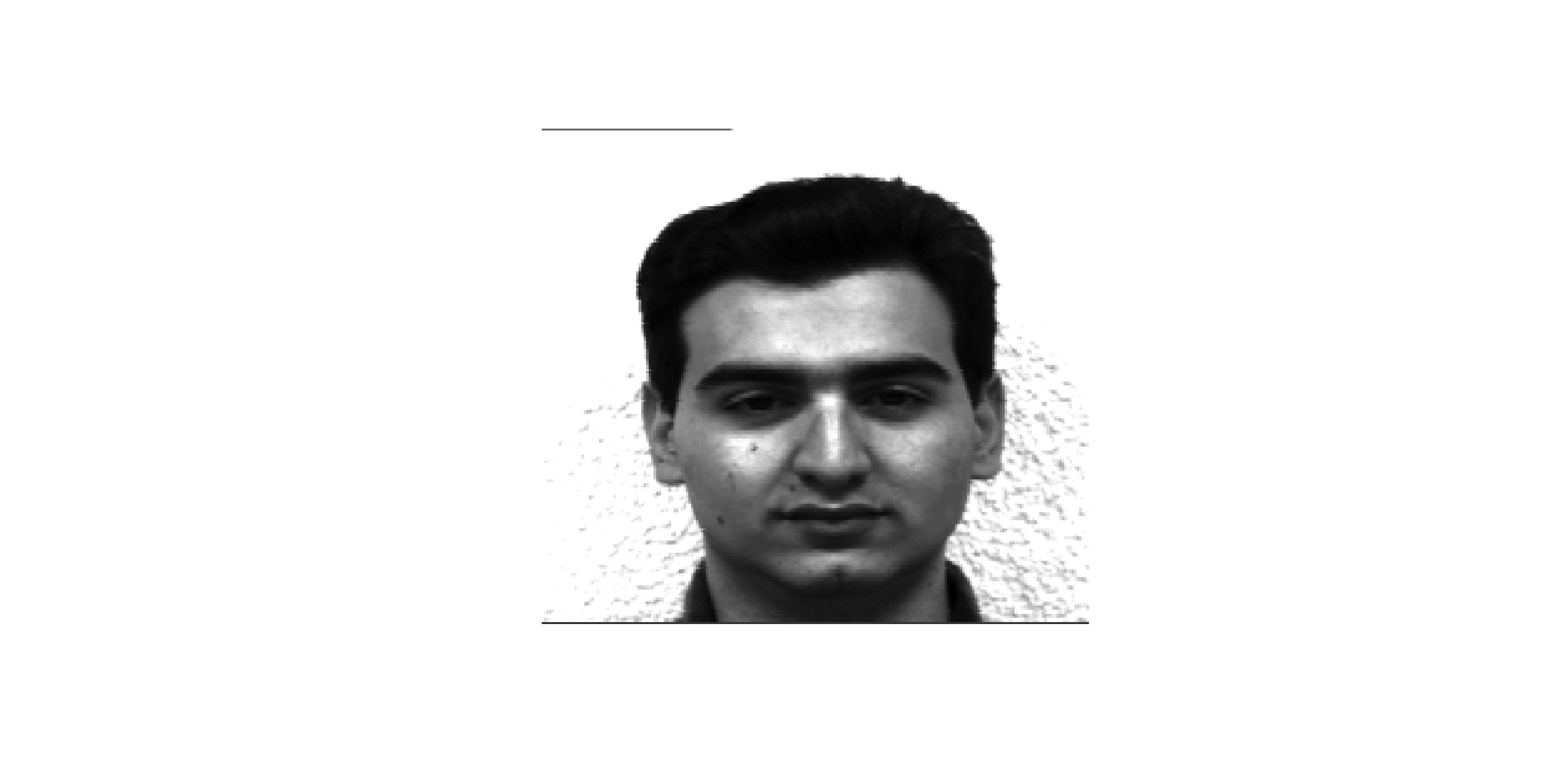
Image = data

• An image (in black and white) can be represented as a data matrix (n rows \times p columns): \underset{n \times p}{X} where the grayscale intensity of each pixel is represented in the corresponding cell of the matrix.

• Lighter colors are associated with higher values, while darker colors are associated with lower values (in the range [0,1])

             V1        V2        V3        V4        V5        V6        V7
 [1,] 0.5098039 0.5098039 0.5098039 0.5098039 0.5098039 0.5098039 0.5098039
 [2,] 1.0000000 1.0000000 1.0000000 1.0000000 1.0000000 1.0000000 1.0000000
 [3,] 1.0000000 1.0000000 1.0000000 1.0000000 1.0000000 1.0000000 1.0000000
 [4,] 1.0000000 1.0000000 1.0000000 1.0000000 1.0000000 1.0000000 1.0000000
 [5,] 1.0000000 1.0000000 1.0000000 1.0000000 1.0000000 1.0000000 1.0000000
 [6,] 1.0000000 1.0000000 1.0000000 1.0000000 1.0000000 1.0000000 1.0000000
 [7,] 1.0000000 1.0000000 1.0000000 1.0000000 1.0000000 1.0000000 1.0000000
 [8,] 1.0000000 1.0000000 1.0000000 1.0000000 1.0000000 1.0000000 1.0000000
 [9,] 1.0000000 1.0000000 1.0000000 1.0000000 1.0000000 1.0000000 1.0000000
[10,] 1.0000000 1.0000000 1.0000000 1.0000000 1.0000000 1.0000000 1.0000000

Image compression

• Original image made by 53460 numbers

• Compressed image made by 4850 numbers

Supervised Versus Unsupervised

The Supervised Learning Problem

• Outcome measurement Y (also called dependent variable, response, target).

• Vector of p predictor measurements X=(X_1,X_2,\ldots,X_p) (also called inputs, regressors, covariates, features, independent variables).

• In the regression problem, Y is quantitative (e.g price, blood pressure).

• In the classification problem, Y takes values in a finite, unordered set (survived/died, digit 0-9, cancer class of tissue sample).

• We have training data (x_1, y_1), \ldots , (x_N , y_N ). These are observations (examples, instances) of these measurements.

Objectives

On the basis of the training data we would like to:

• Accurately predict unseen test cases.

• Understand which inputs affect the outcome, and how.

• Assess the quality of our predictions.

Unsupervised learning

• No outcome variable, just a set of predictors (features) measured on a set of samples.

• Objective is more fuzzy — find groups of samples that behave similarly, find features that behave similarly, find linear combinations of features with the most variation.

• Difficult to know how well your are doing.

• Different from supervised learning, but can be useful as a pre-processing step for supervised learning.

Statistical Learning versus Machine Learning

• Machine learning arose as a subfield of Artificial Intelligence.

• Statistical learning arose as a subfield of Statistics.

• There is much overlap - both fields focus on supervised and unsupervised problems:

• Machine learning has a greater emphasis on large scale applications and prediction accuracy.

• Statistical learning emphasizes models and their interpretability, and precision and uncertainty.

Course text

• The course will cover some of the material in this Springer book (ISLR) published in 2021 (Second Edition).

• Each chapter ends with an R lab, in which examples are developed.

• An electronic version of this book is available from https://www.statlearning.com/

Notation

Wage Data

• Study examines wage data for men in the Atlantic region of the U.S.

• Goal: Understand how age, education and year relate to wages

FIGURE 1.1 ISL

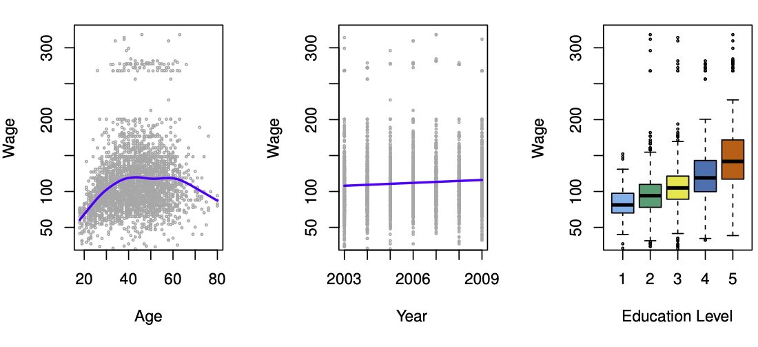
Wage and Age

• Wages increase with age, then decline after ~60

• Relationship is non-linear

• Significant variability: age alone is not a strong predictor

Wage and Year

• Wages increased by about $10,000 from 2003 to 2009

• Trend is roughly linear

• Increase is small relative to overall wage variability

Wage and Education

• Higher education levels are associated with higher wages

• Largest gap between lowest and highest education levels

Notation

Choosing notation is always a difficult task!

• n = number of observations (data points)

• p = number of variables (predictors)

• Example: Wage Data Set

  • n = 3000 individuals

  • p = 11 variables (year, age, race, etc.)

• Variable names are displayed in colored font

	Year	Age	Race	Education	…	Wage
231655	2006	18	White	< HS Grad	…	75.04315
86582	2004	24	White	College Grad	…	70.47602
161300	2003	45	White	Some College	…	130.98218
155159	2003	43	Asian	College Grad	…	154.68529
11443	2005	50	White	HS Grad	…	75.04315
376662	2008	54	White	College Grad	…	127.11574
…	…	…	…	…	…	…

• year Year that wage information was recorded

• age Age of worker

• race A factor with levels 1. White 2. Black 3. Asian and 4. Other indicating race

• education A factor with levels 1. < HS Grad 2. HS Grad 3. Some College 4. College Grad and 5. Advanced Degree indicating education level

• …

• wage Workers raw wage

Indexing Observations and Variables

• x_{ij}: value of the jth variable for the ith observation
• i = 1, \dots, n → indexes observations (rows)
• j = 1, \dots, p → indexes variables (columns)

The Data Matrix \textbf{X}

• \textbf{X} is an n \times p matrix
  
• The (i,j)th element of \textbf{X} is x_{ij}

\textbf{X} = \begin{pmatrix} x_{11} & x_{12} & \dots & x_{1p} \\ x_{21} & x_{22} & \dots & x_{2p} \\ \vdots & \vdots & \ddots & \vdots \\ x_{n1} & x_{n2} & \dots & x_{np} \end{pmatrix}

How to Think About \textbf{X}

• A spreadsheet of numbers
• Rows (n) → observations
  
• Columns (p) → variables
  
• Each cell contains one value x_{ij}

Rows of \textbf{X}

At times we focus on the rows of \textbf{X}, written as
x_1, x_2, \dots, x_n.

Each x_i is a vector of length p, containing the p variable measurements for the ith observation:

x_i = \begin{pmatrix} x_{i1} \\ x_{i2} \\ \vdots \\ x_{ip} \end{pmatrix}

• For the Wage data:
  x_i is a vector of length 11 (year, age, race, etc.) for the ith individual.

Columns of \textbf{X}

We may instead focus on the columns of \textbf{X}, written as \textbf{x}_1, \textbf{x}_2, \dots, \textbf{x}_p.

Each \textbf{x}_j is a vector of length n:

\textbf{x}_j = \begin{pmatrix} x_{1j} \\ x_{2j} \\ \vdots \\ x_{nj} \end{pmatrix}

• For the Wage data:
  \textbf{x}_1 contains the n = 3000 values of year.

Alternative Representations of \textbf{X}

Using column notation:

\textbf{X} = \begin{pmatrix} \textbf{x}_1 & \textbf{x}_2 & \cdots & \textbf{x}_p \end{pmatrix}

Using row notation:

\textbf{X} = \begin{pmatrix} x_1^{T} \\ x_2^{T} \\ \vdots \\ x_n^{T} \end{pmatrix}

Transpose Notation

The superscript T denotes the transpose of a vector or matrix.

\textbf{X}^{T} = \begin{pmatrix} x_{11} & x_{21} & \dots & x_{n1} \\ x_{12} & x_{22} & \dots & x_{n2} \\ \vdots & \vdots & \ddots & \vdots \\ x_{1p} & x_{2p} & \dots & x_{np} \end{pmatrix}

while the transpose of x_i is a row vector:

x_i^{T} = \begin{pmatrix} x_{i1} & x_{i2} & \cdots & x_{ip} \end{pmatrix}

Response Variable

We use y_i to denote the ith observation of the variable we wish to predict (e.g., wage).

The response vector is written as:

\mathbf{y} = \begin{pmatrix} y_1 \\ y_2 \\ \vdots \\ y_n \end{pmatrix}

Our observed data consists of:

\{(x_1, y_1), (x_2, y_2), \dots, (x_n, y_n)\}

where each x_i is a vector of length p.
(If p = 1, then x_i is simply a scalar.)

Notation Conventions

• Vectors of length n → lowercase bold

  \mathbf{a} = \begin{pmatrix} a_1 \\ a_2 \\ \vdots \\ a_n \end{pmatrix}

• Vectors not of length n (e.g., feature vectors of length p) → lowercase normal font, e.g. a

• Scalars → lowercase normal font, e.g. a

• Matrices → bold capital letters, e.g. \textbf{A}

• Random variables → capital normal font, e.g. A

Indicating Dimensions

Occasionally we indicate the dimension of an object using set notation.

• Scalar: a \in \mathbb{R}

• Vector of length k: a \in \mathbb{R}^k

• Vector of length n: \textbf{a} \in \mathbb{R}^n

• r \times s matrix: \textbf{A} \in \mathbb{R}^{r \times s}

Required readings from the textbook and course materials

• Chapter 1: Introduction

• Chapter 2: Statistical Learning

  • 2.1 What Is Statistical Learning?
    • 2.1.1 Why Estimate f?
    • 2.1.2 How Do We Estimate f?
    • 2.1.3 The Trade-Off Between Prediction Accuracy and Model Interpretability
    • 2.1.4 Supervised Versus Unsupervised Learning
    • 2.1.5 Regression Versus Classification Problems

Video SL 1.1 Opening Remarks - 18:19
Video SL 1.2 Examples and Framework - 12:13
Video SL 2.1 Introduction to Regression Models - 11:42
Video SL 2.2 Dimensionality and Structured Models - 11:41