| Volume | Diameter | Height |
|---|---|---|
| 10.3 | 8.3 | 70 |
| 10.3 | 8.6 | 65 |
| 10.2 | 8.8 | 63 |
| 16.4 | 10.5 | 72 |
| 18.8 | 10.7 | 81 |
| 19.7 | 10.8 | 83 |
Linear Regression
Introduction to Statistical Learning - PISE
This unit will cover the following topics:
- Linear models
- The modeling process
Trees data
These data give the
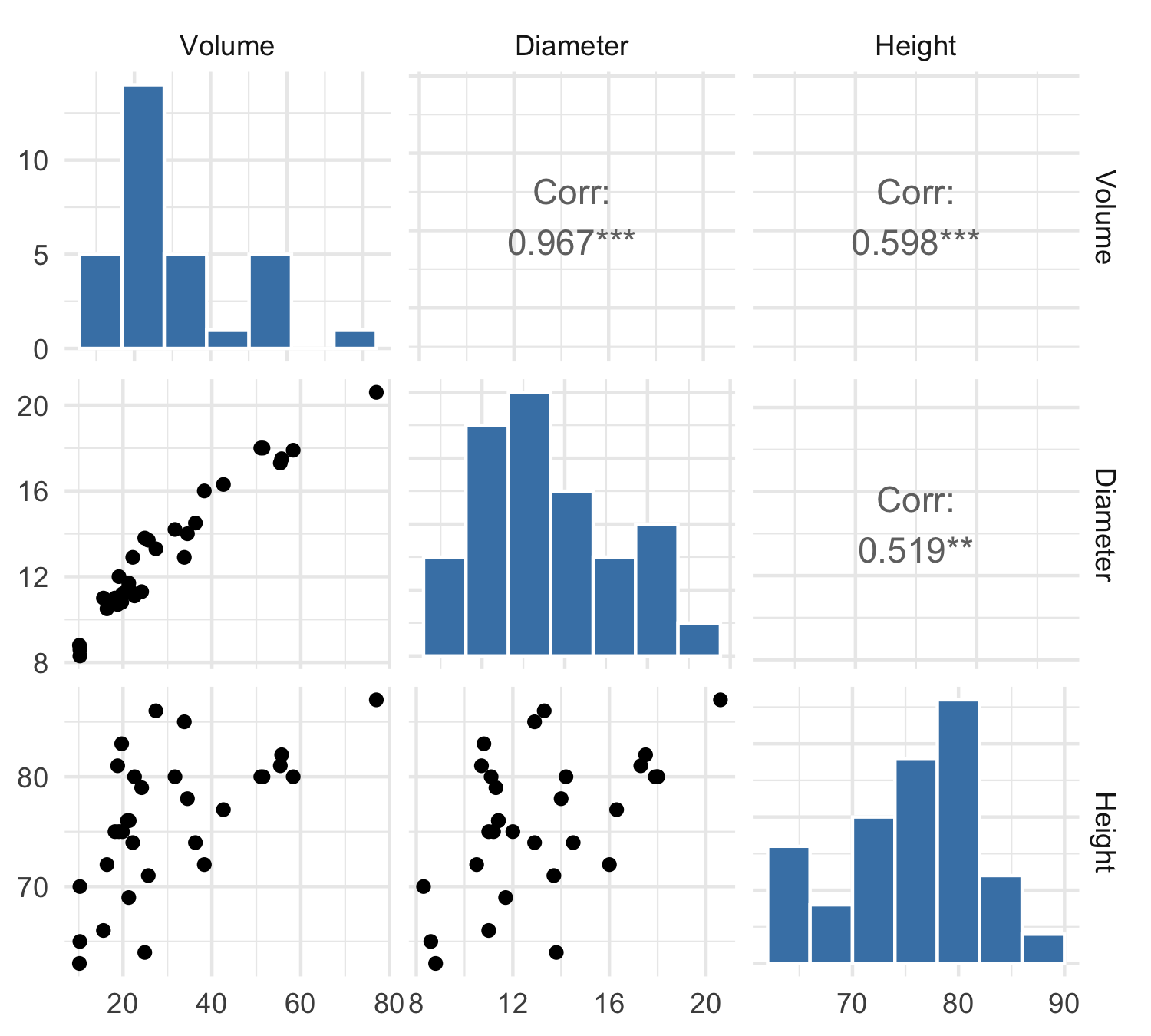
Volume(cubic feet),Height(feet) andDiameter(inches) (at 54 inches above ground) for a sample of n=31 black cherry trees in the Allegheny National Forest, Pennsylvania.The data were collected in order to find an estimate for the volume of a tree Y (and therefore for the timber yield), given its diameter X_1 and height X_2.
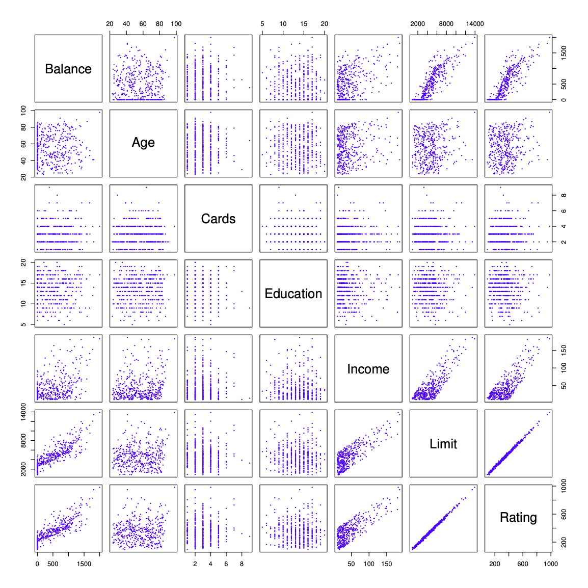
Scatterplot Matrix
Scatterplot 3d
Multiple linear regression
Linear regression is a simple approach to supervised learning. It assumes that the dependence of Y on X_1,X_2,\ldots,X_p is linear.
The linear model is given by Y = \beta_0 + \beta_1X_1 + \beta_2 X_2 + \ldots + \beta_p X_p + \varepsilon
Given estimates \hat{\beta}_0,\hat{\beta}_1,\ldots,\hat{\beta}_p we can make predictions using the formula \hat{y} = \hat\beta_0 + \hat\beta_1 x_1 + \hat\beta_2 x_2 + \ldots + \hat\beta_p x_p
We estimate \beta_0,\beta_1,\ldots,\beta_p as the values that minimize the sum of squared residuals
\mathrm{RSS} = \sum_{i=1}^{n} (y_i - \hat y_i)^2= \sum_{i=1}^{n} (y_i - \hat{\beta}_0- \hat{\beta}_1 x_{i1}- \hat{\beta}_2 x_{i2}- \ldots - \hat{\beta}_p x_{ip})^2
- This is done using standard statistical software. The values \hat{\beta}_0,\hat{\beta}_1,\ldots,\hat{\beta}_p that minimize RSS are the least squares estimates.
Interpreting regression coefficients
We interpret \beta_j as the average effect on Y of a one unit increase in X_j, holding all other predictors fixed
But predictors usually change together! For example, in the tree data, larger
Diameteris typically associated with greaterHeight. HoldingHeightfixed while increasingDiametermay be unrealistic.
Model 1: Volume ~ Diameter + Height
\mathrm{Volume} = \beta_0 + \beta_1 \times \mathrm{Diameter} + \beta_2 \times \mathrm{Height} + \varepsilon
| Estimate | Std_Error | t_value | p_value | |
|---|---|---|---|---|
| (Intercept) | -57.9877 | 8.6382 | -6.7129 | 0.0000 |
| Diameter | 4.7082 | 0.2643 | 17.8161 | 0.0000 |
| Height | 0.3393 | 0.1302 | 2.6066 | 0.0145 |
MSE training: 13.6104R^2 training: 0.9480Model 1: Regression plane
Potential Problems
When we fit a linear regression model to a particular data set, many problems may occur. Most common among these are the following:
Non-linearity of the response-predictor relationships.
Correlation of error terms.
Non-constant variance of error terms.
Outliers.
High-leverage points.
Collinearity.
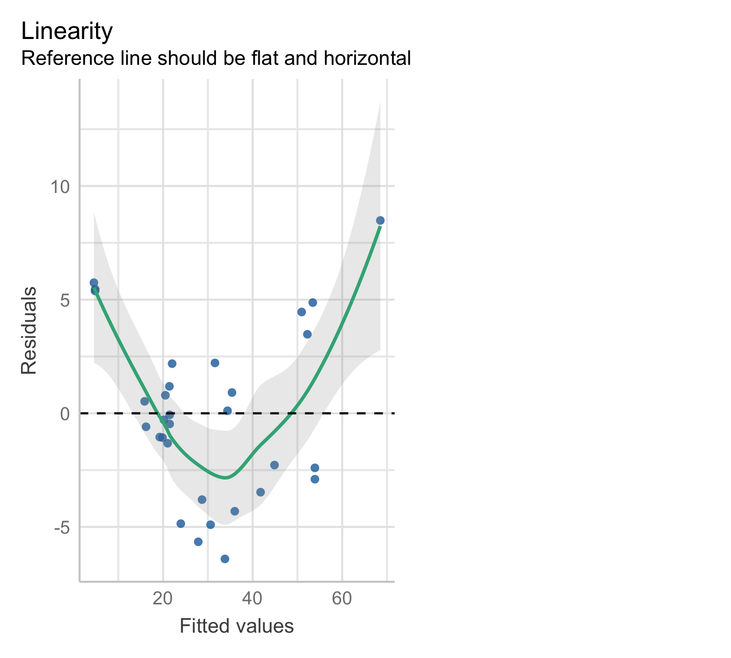
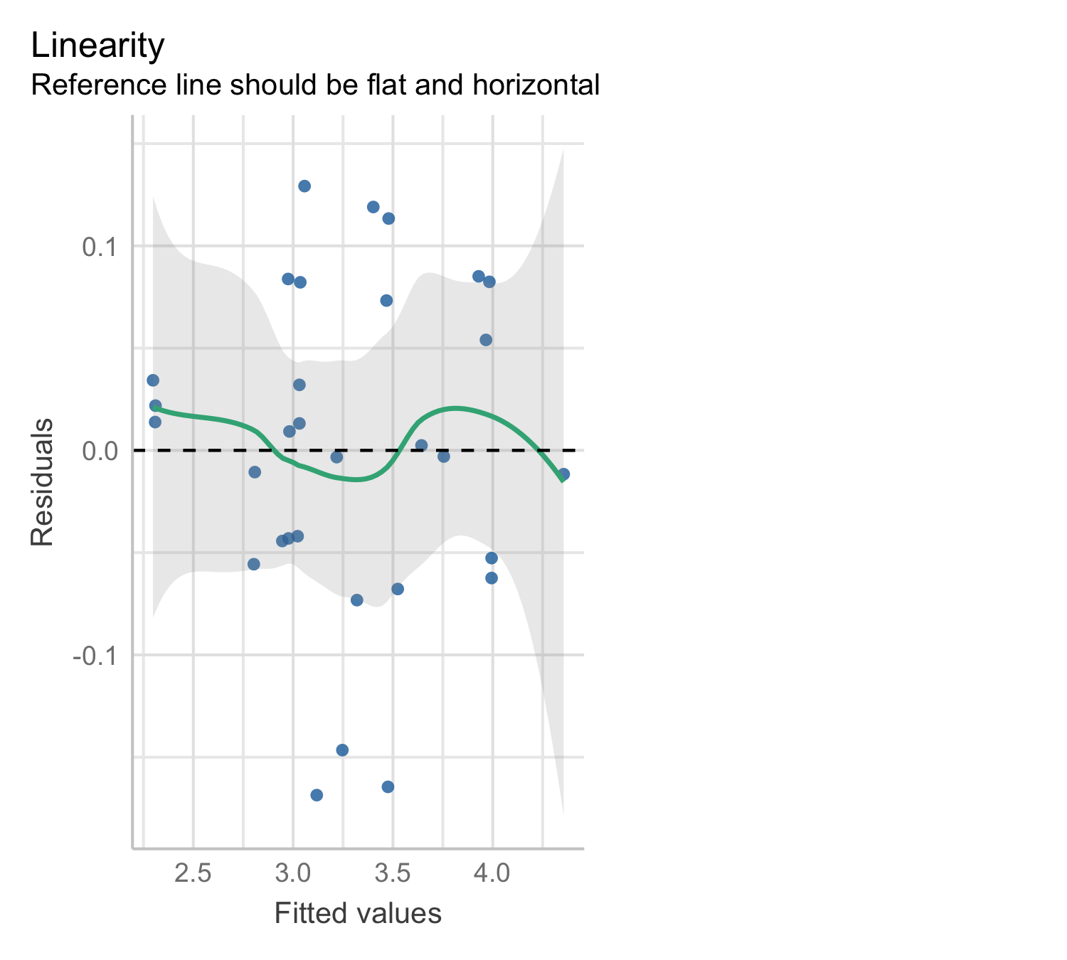
Residual plot
Residual plots are a useful graphical tool for identifying non-linearity
Plot the residuals, e_i = y_i - \hat{y}_i, against the fitted values \hat{y}_i.
A systematic pattern in this plot may indicate violations of the linearity assumption
Model 1: residual plot
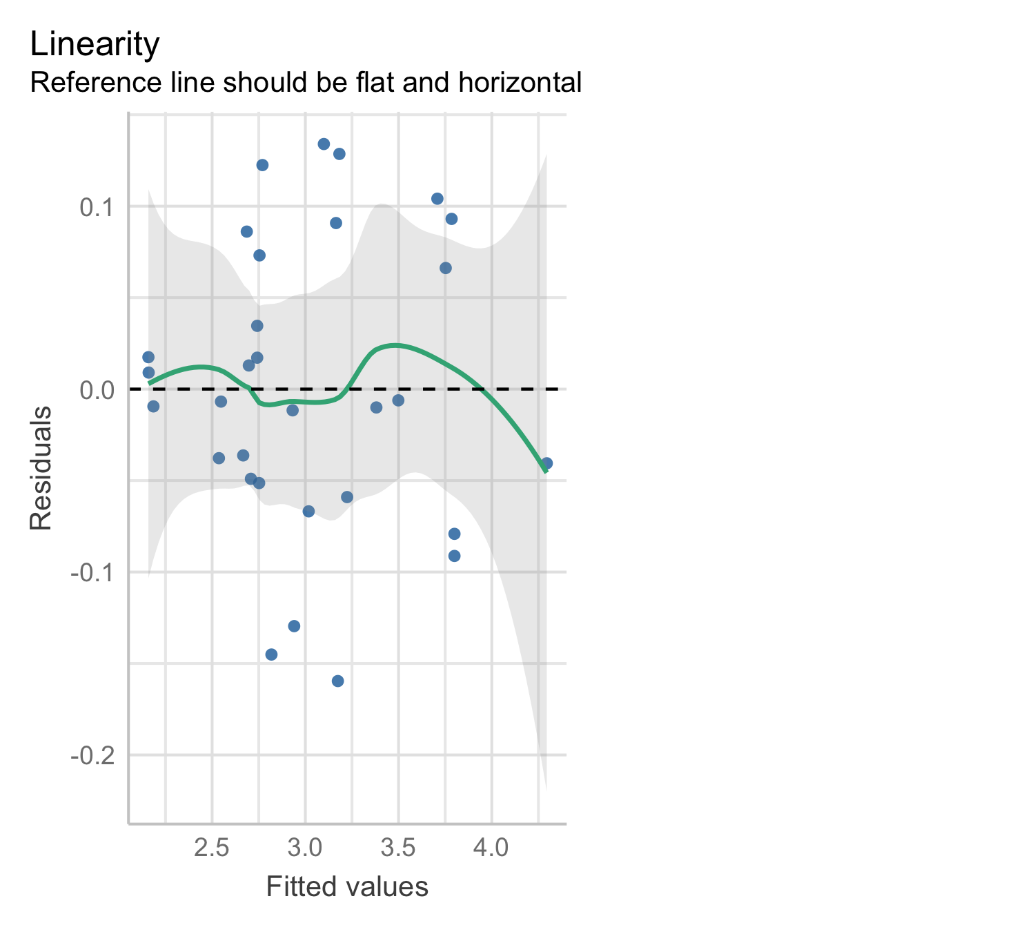
Model 2: Cube-root transformation of the response
A cube-root transformation of the response leads to the model \mathrm{Volume}^{1/3} = \beta_0 + \beta_1 \times \mathrm{Diameter} + \beta_2 \times \mathrm{Height} + \varepsilon in which both sides have the dimension of length.
After fitting the model, we obtain the predicted cube-root volume
\widehat{\mathrm{Volume}^{1/3}} = \hat\beta_0 + \hat\beta_1 \mathrm{Diameter} + \hat\beta_2 \mathrm{Height}.
- To predict
Volumeon the original scale, we cube the fitted value:
\widehat{\mathrm{Volume}} = \left( \widehat{\mathrm{Volume}^{1/3}} \right)^3.
Model 2: predicted surface
Model 2: residual plot
Check model assumptions (residual plot) on the fitting scale:
Model 2: goodness-of-fit
Compare the goodness-of-fit (training MSE and R^2) after converting predictions back to the original Y-scale:
\mathrm{MSE_{trasformed}} = \frac{1}{n}\sum_{i=1}^{n} (y_i^{1/3} - \widehat{y^{1/3}_i} )^2,\qquad \mathrm{MSE_{original}} = \frac{1}{n}\sum_{i=1}^{n} (y_i - (\widehat{y^{1/3}_i})^3 )^2 and \mathrm{R^2_{trasformed}} = 1-\frac{\sum_{i=1}^{n} ( y_i^{1/3} - \widehat{y^{1/3}_i} )^2 }{ \sum_{i=1}^{n} (y_i^{1/3} - \overline{y^{1/3}} )^2}, \qquad \mathrm{R^2_{original}} = 1-\frac{\sum_{i=1}^{n} ( y_i - (\widehat{y^{1/3}_i})^3 )^2 }{ \sum_{i=1}^{n} (y_i - \bar y )^2}
MSE original: 0.0062R^2 trasformed: 0.9777MSE original: 5.9603R^2 original: 0.9772Trees as cylinders
A tree trunk can be viewed as a cylinder (or a cone): \mathrm{Volume} = (\text{Area of base}) \times (\text{Height}). Since the base area is proportional to the square of the diameter, \text{Area of base} = \pi \left(\frac{\mathrm{Diameter}}{2}\right)^2 we obtain \mathrm{Volume} = \frac{\pi}{4} \times \mathrm{Diameter}^2 \times \mathrm{Height}.
Model 3: transformation of the predictors
The previous reasoning suggests the regression model \mathrm{Volume} = \beta \times \mathrm{Diameter}^2 \times \mathrm{Height} + \varepsilon, where \beta = \frac{\pi}{4} or \beta = \frac{\pi}{12} if trees were perfect cylinder or cones.
| Estimate | Std_Error | t_value | p_value |
|---|---|---|---|
| 0.0021 | 0 | 77.4365 | 0 |
Model 3 predicted line
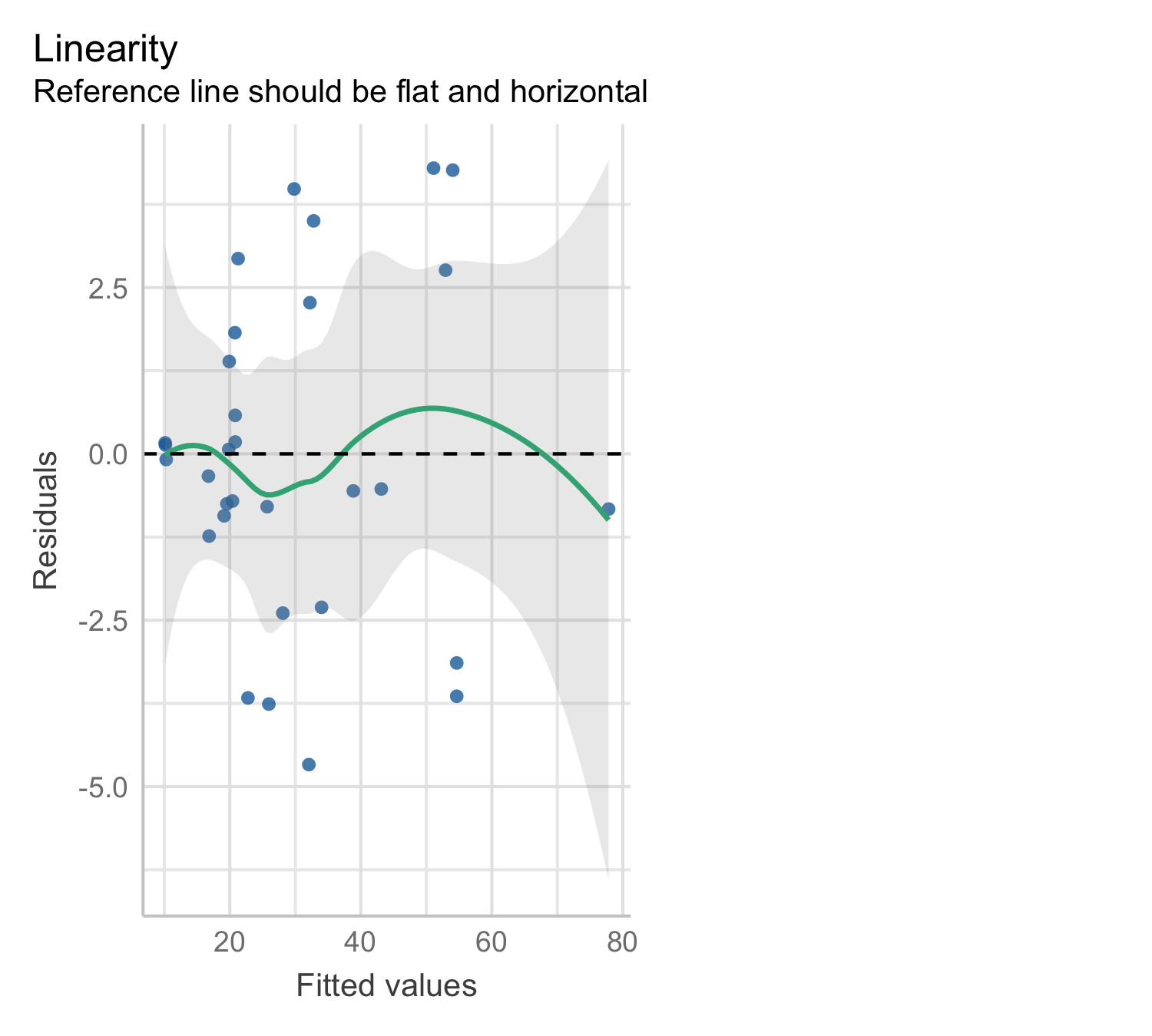
Model 3: residual plot

Model 4: Log–Log Transformation
Model 4 applies a logarithmic transformation to both the response and predictors:
\log \mathrm{Volume} = \beta_0 + \beta_1 \times \log \mathrm{Diameter} + \beta_2 \times \log \mathrm{Height} + \varepsilon.
For the tree data, geometry suggests
\mathrm{Volume} = \beta \times \mathrm{Diameter}^2 \times \mathrm{Height},
and taking logs gives
\log \mathrm{Volume} = \log \beta + 2 \times \log \mathrm{Diameter} + 1 \times \log \mathrm{Height}, Thus the log–log specification allows the exponents to be estimated from the data.
| Estimate | Std_Error | t_value | p_value | |
|---|---|---|---|---|
| (Intercept) | -6.6316 | 0.7998 | -8.2917 | 0 |
| log(Diameter) | 1.9826 | 0.0750 | 26.4316 | 0 |
| log(Height) | 1.1171 | 0.2044 | 5.4644 | 0 |
Model 4: residual plot
Modelling the Log Response
- Consider the linear model for the log response with p predictors:
\log Y = \beta_0 + \beta_1 X_1 + \cdots + \beta_p X_p + \varepsilon.
If \varepsilon \sim N(0,\sigma^2), then \log Y \mid X \sim N(\mu,\sigma^2), where \mu = \beta_0 + \beta_1 X_1 + \cdots + \beta_p X_p and X=(X_1,\dots,X_p)^T.
Then Y \mid X \sim \text{Lognormal}(\mu,\sigma^2). For a lognormal random variable: \text{Median}(Y \mid X) = \exp(\mu), \qquad \mathbb{E}(Y \mid X) = \exp(\mu + \sigma^2/2).
Thus \exp(\hat\mu)= \exp(\hat\beta_0+\hat\beta_1 X_1+\cdots+\hat\beta_p X_p) estimates \text{Median}(Y \mid X), while \mathbb{E}(Y \mid X) is larger because the distribution of Y|X is right-skewed.
To estimate \mathbb{E}(Y \mid X), use
\exp(\hat\mu)\exp(\hat\sigma^2/2).
Model comparison
To compare the three models using LOOCV (leave-one-out cross-validation) on the original Volume scale, we:
Leave one tree out
Fit the model on the remaining 30 observations
Predict the left-out tree
Compute squared error on the original Volume (ft³) scale
Repeat for all 31 trees
Compare root mean squared prediction error (LOOCV RMSE)
| Model | LOOCV_MSE | LOOCV_RMSE | |
|---|---|---|---|
| Model1 | Baseline | 18.158 | 4.261 |
| Model2 | Cube-root | 7.314 | 2.705 |
| Model3 | Cylinder | 6.399 | 2.530 |
| Model4 | Log-Log | 6.984 | 2.643 |
| Model4bc | Log-Log (bias-corrected) | 6.958 | 2.638 |
Credit data
The response variable is
Balance(average credit card debt for each individual).The quantitative predictors are:
Age— age in yearsCards— number of credit cardsEducation— years of educationIncome— income (in thousands of dollars)Limit— credit limitRating— credit rating
Figure 3.6 ISL
Qualitative Predictors
Some predictors are not quantitative but qualitative, meaning they take values from a discrete set of categories.
These are also called categorical predictors or factor variables.
In regression, qualitative predictors must be represented using indicator (dummy) variables.
In the Credit data, in addition to the seven quantitative variables shown in the scatterplot matrix, there are four qualitative variables:
Gender
Student(student status)
Married(marital status)
Ethnicity(Caucasian, African American, or Asian)
Qualitative Predictors - continued
- For example,
Ethnicityhas three levels, and we create two dummy variables:
x_{i1} = \begin{cases} 1 & \text{if the } i\text{th person is Asian} \\ 0 & \text{otherwise} \end{cases}, \qquad x_{i2} = \begin{cases} 1 & \text{if the } i\text{th person is Caucasian} \\ 0 & \text{otherwise} \end{cases}
- The regression model, ignoring the other variables, becomes
y_i = \beta_0 + \beta_1 x_{i1} + \beta_2 x_{i2} + \varepsilon_i.
- This implies
y_i = \begin{cases} \beta_0 + \beta_1 + \varepsilon_i & \text{if Asian} \\ \beta_0 + \beta_2 + \varepsilon_i & \text{if Caucasian} \\ \beta_0 + \varepsilon_i & \text{if African American} \end{cases}
There is always one fewer dummy variable than the number of levels.
The level without a dummy variable (African American here) is called the baseline level.
The coefficients \beta_1 and \beta_2 measure differences relative to the baseline.
| Estimate | Std. Error | t value | Pr(>|t|) | |
|---|---|---|---|---|
| (Intercept) | 531.000 | 46.319 | 11.464 | 0.000 |
| EthnicityAsian | -18.686 | 65.021 | -0.287 | 0.774 |
| EthnicityCaucasian | -12.503 | 56.681 | -0.221 | 0.826 |
Interactions between qualitative and quantitative variables
Consider the Credit data set. Suppose we wish to predict
Balance using Income (quantitative) and
Student (qualitative).
Define an indicator variable x_i = \begin{cases} 1 & \text{if the } i\text{th person is a student} \\ 0 & \text{otherwise} \end{cases}
Without an interaction term, the model is \text{balance}_i = \beta_0 + \beta_1 \text{income}_i +\beta_2 x_i+\varepsilon_i.
This implies
\text{balance}_i = \begin{cases} (\beta_0 + \beta_2) + \beta_1 \text{income}_i + \varepsilon_i & \text{if student} \\ \beta_0 + \beta_1 \text{income}_i + \varepsilon_i & \text{if not student} \end{cases}
Include an interaction between Income and Student:
\text{balance}_i = \beta_0 + \beta_1 \text{income}_i + \beta_2 x_i + \beta_3 (\text{income}_i x_i) + \varepsilon_i,
This implies
\text{balance}_i = \begin{cases} (\beta_0 + \beta_2) + (\beta_1 + \beta_3)\text{income}_i + \varepsilon_i & \text{if student} \\ \beta_0 + \beta_1 \text{income}_i + \varepsilon_i & \text{if not student} \end{cases}
- Intercepts differ.
- Slopes differ.
- The effect of income on balance depends on student status.
Figure 3.7 ISL
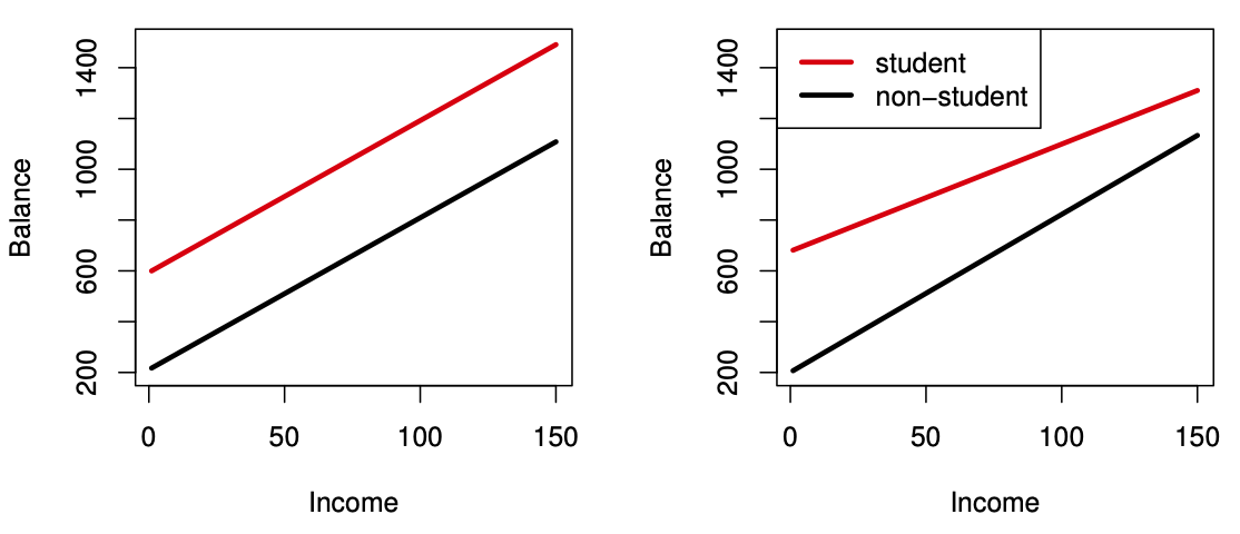
Credit data; Left: no interaction between Income and Student. Right: with an interaction term between Income and Student.
Subset Selection
For deciding on the important variables, the most direct approach is called best subsets regression: we compute the least squares fit for all possible subsets and then choose between them based on some criterion that balances training error with model size.
However we often can’t examine all possible models, since they are 2^p of them; for example when p= 40 there are over a billion models!
Best Subset Selection
Let \mathcal M_0 denote the null model, which contains no predictors. This model predicts the sample mean of the response for all observations.
For k = 1, 2, \dots, p:
- Fit all \binom{p}{k} models that contain exactly k predictors.
- Fit all \binom{p}{k} models that contain exactly k predictors.
- Among these, select the best model and call it \mathcal M_k.
``Best’’ is typically defined as the model with the smallest RSS
(equivalently, the largest R^2).
- Among these, select the best model and call it \mathcal M_k.
From the models \mathcal M_0, \mathcal M_1, \dots, \mathcal M_p, choose a final model using cross-validated prediction error, Cp (AIC), BIC, or adjusted R^2
Figure 6.1 ISL
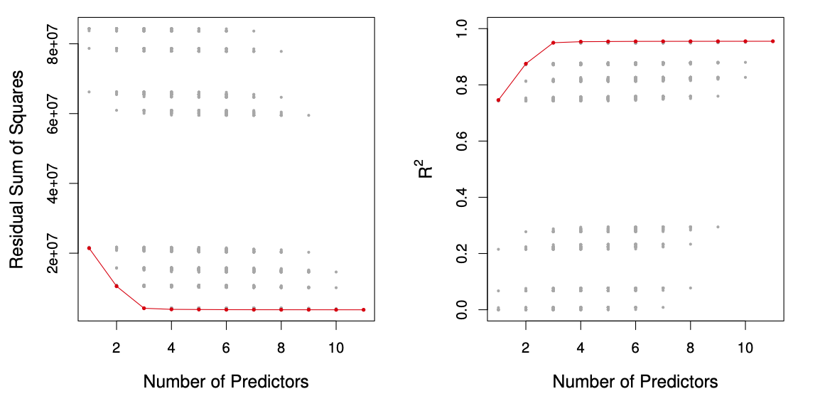
For each possible model containing a subset of the ten predictors in the Credit data set, the RSS and R^2 are displayed. The red frontier tracks the best model for a given number of predictors, according to RSS and R^2. Though the data set contains only ten predictors, the x-axis ranges from 1 to 11, since one of the variables is categorical and takes on three values, leading to the creation of two dummy variables.
Forward Stepwise Selection
Forward stepwise selection starts with the null model (no predictors).
Predictors are added one at a time.
At each step, the predictor that provides the greatest additional improvement in model fit is added.
The procedure continues until all predictors are included.
Forward Stepwise Selection — In Detail
Let \mathcal M_0 denote the null model (no predictors).
For k = 0, 1, \dots, p-1:
- Consider all p - k models formed by adding one new predictor to M_k.
- Among these models, choose the best and call it \mathcal M_{k+1}. ``Best’’ is typically defined as the model with the smallest RSS (equivalently, the largest R^2).
From the sequence of models \mathcal M_0, \mathcal M_1, \dots, \mathcal M_p, select a final model using cross-validated prediction error, Cp (AIC), BIC, or adjusted R^2
Credit data example
The first four selected models using best subset selection and forward stepwise selection:
| # Variables | Best Subset | Forward Stepwise |
|---|---|---|
| One | rating |
rating |
| Two | rating, income |
rating, income |
| Three | rating, income, student |
rating, income, student |
| Four | cards, income, student, limit |
rating, income, student, limit |
The first four selected models for best subset selection and forward stepwise selection on the Credit data set. The first three models are identical but the fourth models differ.
Choosing the Optimal Model
The model containing all of the predictors will always have the smallest RSS and the largest R^2, since these quantities are related to the training error.
We wish to choose a model with low test error, not a model with low training error. Recall that training error is usually a poor estimate of test error.
Therefore, RSS and R^2 are not suitable for selecting the best model among a collection of models with different numbers of predictors.
Estimating test error: two approaches
We can indirectly estimate test error by making an adjustment to the training error to account for the bias due to overfitting.
We can directly estimate the test error, using either a validation set approach or a cross-validation approach, as discussed in previous lectures
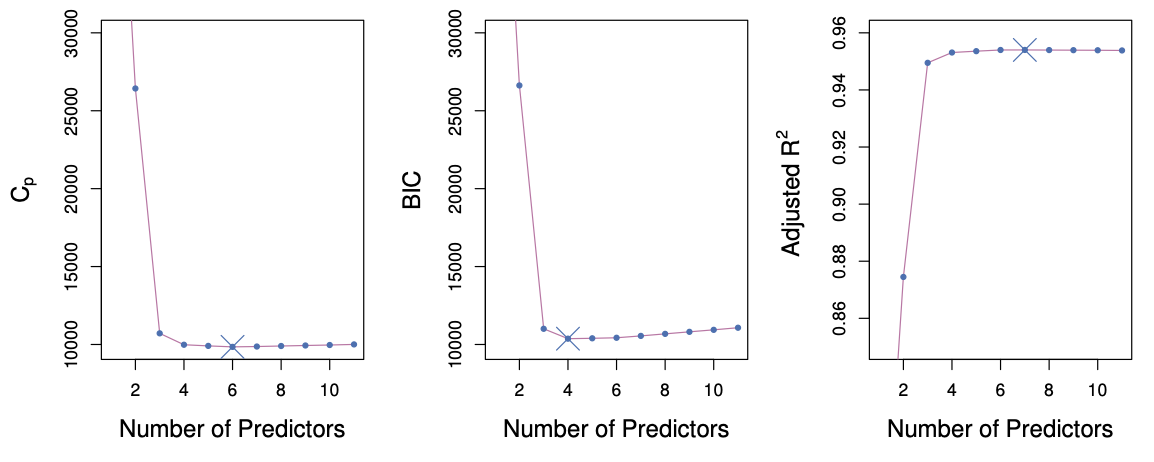
C_p, AIC, BIC, and Adjusted R^2
These techniques adjust the training error for model size, and can be used to select among a set of models with different numbers of variables.
The next figure displays C_p, BIC, and adjusted R^2 for the best model of each size produced by best subset selection on the
Creditdata set.
Figure 6.2 ISL
Mallows’ C_p
C_p = \frac{1}{n} \left( \text{RSS} + 2 d \hat{\sigma}^2 \right),
where d is the total number of parameters used and \hat{\sigma}^2 is an estimate of the variance of the error \varepsilon associated with each response measurement.
BIC
\text{BIC} = \frac{1}{n} \left( \text{RSS} + \log(n)\, d \hat{\sigma}^2 \right).
Like C_p, the Bayesian Information Criterion (BIC) tends to be small for models with low test error.
We typically select the model with the lowest BIC.Notice that BIC replaces the 2 d \hat{\sigma}^2 term used by C_p with a \log(n)\, d \hat{\sigma}^2 term, where n is the number of observations.
Since \log(n) > 2 for any n > 7, BIC generally places a heavier penalty on models with many variables.
As a result, BIC tends to select smaller models than C_p.
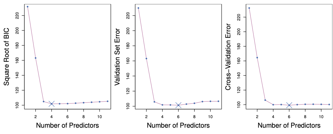
Validation and Cross-Validation
Each model selection procedure returns a sequence of models \mathcal M_k indexed by model size k = 0, 1, 2, \dots. Our goal is to choose \hat{k}.
Once selected, we return the model \mathcal M_{\hat{k}}.We compute the validation set error or the cross-validation error for each model \mathcal M_k, and select the value of k for which the estimated test error is smallest.
This approach has an advantage over AIC, BIC, C_p, and adjusted R^2: it provides a direct estimate of test error and does not require an estimate of the error variance \sigma^2.
It can also be applied in a wider range of model selection problems, including settings where the model degrees of freedom are difficult to determine or where estimating \sigma^2 is challenging.
Figure 6.3 ISL
Required readings from the textbook and course materials
- Chapter 3: Linear Regression
- 3.1 Simple Linear Regression
- 3.1.1 Estimating the Coefficients
- 3.1.3 Assessing the Accuracy of the Model
- 3.2 Multiple Linear Regression
- 3.2.1 Estimating the Regression Coefficients
- 3.3 Other Considerations in the Regression Model
- 3.3.1 Qualitative Predictors
- 3.1 Simple Linear Regression
- Chapter 6: Linear Model Selection and Regularization
- 6.1 Subset Selection
- 6.1.1 Best Subset Selection
- 6.1.2 Stepwise Selection
- 6.1.3 Choosing the Optimal Model
- 6.1 Subset Selection
Required readings from the textbook and course materials
Video SL 3.1 Simple Linear Regression - 13:02
Video SL 3.3 Multiple Linear Regression - 15:38
Video SL 3.4 Some Important Questions - 14:52
Video SL 3.5 Extensions of the Linear Model - 14:17
Video SL 6.1 Introduction and Best Subset Selection - 13:45
Video SL 6.3 Backward Stepwise Selection - 5:27