Lab 2

Introduction to Statistical Learning - PISE

Author

Affiliation

Aldo Solari

Ca’ Foscari University of Venice

Linear Regression

Libraries

• library() loads packages
  
• Packages contain functions and datasets not always included in base R
  
• Basic linear regression tools are in base R
  
• More specialized tools require additional packages
  
• Here we load:
  • MASS
  • ISLR2

library(MASS)
library(ISLR2)

Attaching package: 'ISLR2'

The following object is masked from 'package:MASS':

    Boston

• If a package is not installed, library() returns an error
  
• Some packages (e.g. MASS) usually come with R
  
• Others (e.g. ISLR2) may need to be installed first
  
• Install once with install.packages("ISLR2")
  
• Then load the package in each new R session with library()

Simple Linear Regression

• Boston is a dataset in ISLR2
  
• Response variable: medv (median house value)
  
• Predictors include variables such as:
  • rm
  • age
  • lstat

head(Boston)

     crim zn indus chas   nox    rm  age    dis rad tax ptratio lstat medv
1 0.00632 18  2.31    0 0.538 6.575 65.2 4.0900   1 296    15.3  4.98 24.0
2 0.02731  0  7.07    0 0.469 6.421 78.9 4.9671   2 242    17.8  9.14 21.6
3 0.02729  0  7.07    0 0.469 7.185 61.1 4.9671   2 242    17.8  4.03 34.7
4 0.03237  0  2.18    0 0.458 6.998 45.8 6.0622   3 222    18.7  2.94 33.4
5 0.06905  0  2.18    0 0.458 7.147 54.2 6.0622   3 222    18.7  5.33 36.2
6 0.02985  0  2.18    0 0.458 6.430 58.7 6.0622   3 222    18.7  5.21 28.7

• Use ?Boston to see the dataset documentation

• Fit a simple linear regression with lm()
  

• Syntax: lm(y ~ x, data = dataset)
  

• Here:

  • response = medv
  • predictor = lstat

lm.fit <- lm(medv ~ lstat)

Error in eval(predvars, data, env): object 'medv' not found

• This gives an error because R does not know where medv and lstat are stored
  
• Fix:
  • specify data = Boston, or
  • use attach(Boston)

lm.fit <- lm(medv ~ lstat, data = Boston)
attach(Boston)
lm.fit <- lm(medv ~ lstat)

• Typing lm.fit gives basic model output
  
• summary(lm.fit) gives more details:
  • coefficients
  • standard errors
  • p-values
  • R^2
  • F-statistic

lm.fit

Call:
lm(formula = medv ~ lstat)

Coefficients:
(Intercept)        lstat  
      34.55        -0.95  

summary(lm.fit)

Call:
lm(formula = medv ~ lstat)

Residuals:
    Min      1Q  Median      3Q     Max 
-15.168  -3.990  -1.318   2.034  24.500 

Coefficients:
            Estimate Std. Error t value Pr(>|t|)    
(Intercept) 34.55384    0.56263   61.41   <2e-16 ***
lstat       -0.95005    0.03873  -24.53   <2e-16 ***
---
Signif. codes:  0 '***' 0.001 '**' 0.01 '*' 0.05 '.' 0.1 ' ' 1

Residual standard error: 6.216 on 504 degrees of freedom
Multiple R-squared:  0.5441,    Adjusted R-squared:  0.5432 
F-statistic: 601.6 on 1 and 504 DF,  p-value: < 2.2e-16

• Use names() to see what is stored in the fitted model object
  
• Use extractor functions such as coef() to access components safely

names(lm.fit)

 [1] "coefficients"  "residuals"     "effects"       "rank"         
 [5] "fitted.values" "assign"        "qr"            "df.residual"  
 [9] "xlevels"       "call"          "terms"         "model"        

coef(lm.fit)

(Intercept)       lstat 
 34.5538409  -0.9500494 

• Use confint() to compute confidence intervals for coefficients

confint(lm.fit)

                2.5 %     97.5 %
(Intercept) 33.448457 35.6592247
lstat       -1.026148 -0.8739505

• Use predict() to compute:
  • confidence intervals for the mean response
  • prediction intervals for a new observation

predict(lm.fit, data.frame(lstat = (c(5, 10, 15))),
    interval = "confidence")

       fit      lwr      upr
1 29.80359 29.00741 30.59978
2 25.05335 24.47413 25.63256
3 20.30310 19.73159 20.87461

predict(lm.fit, data.frame(lstat = (c(5, 10, 15))),
    interval = "prediction")

       fit       lwr      upr
1 29.80359 17.565675 42.04151
2 25.05335 12.827626 37.27907
3 20.30310  8.077742 32.52846

• Confidence and prediction intervals are centered at the same fitted value
  

• Prediction intervals are wider than confidence intervals

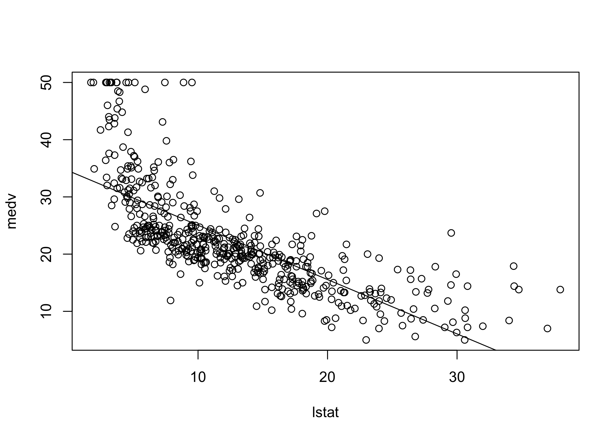
• Plot the data and add the least-squares regression line

plot(lstat, medv)
abline(lm.fit)

• The plot suggests some possible non-linearity
  

• We will revisit this later

• abline() can add any line to a plot
  

• abline(a, b) draws a line with:

  • intercept = a
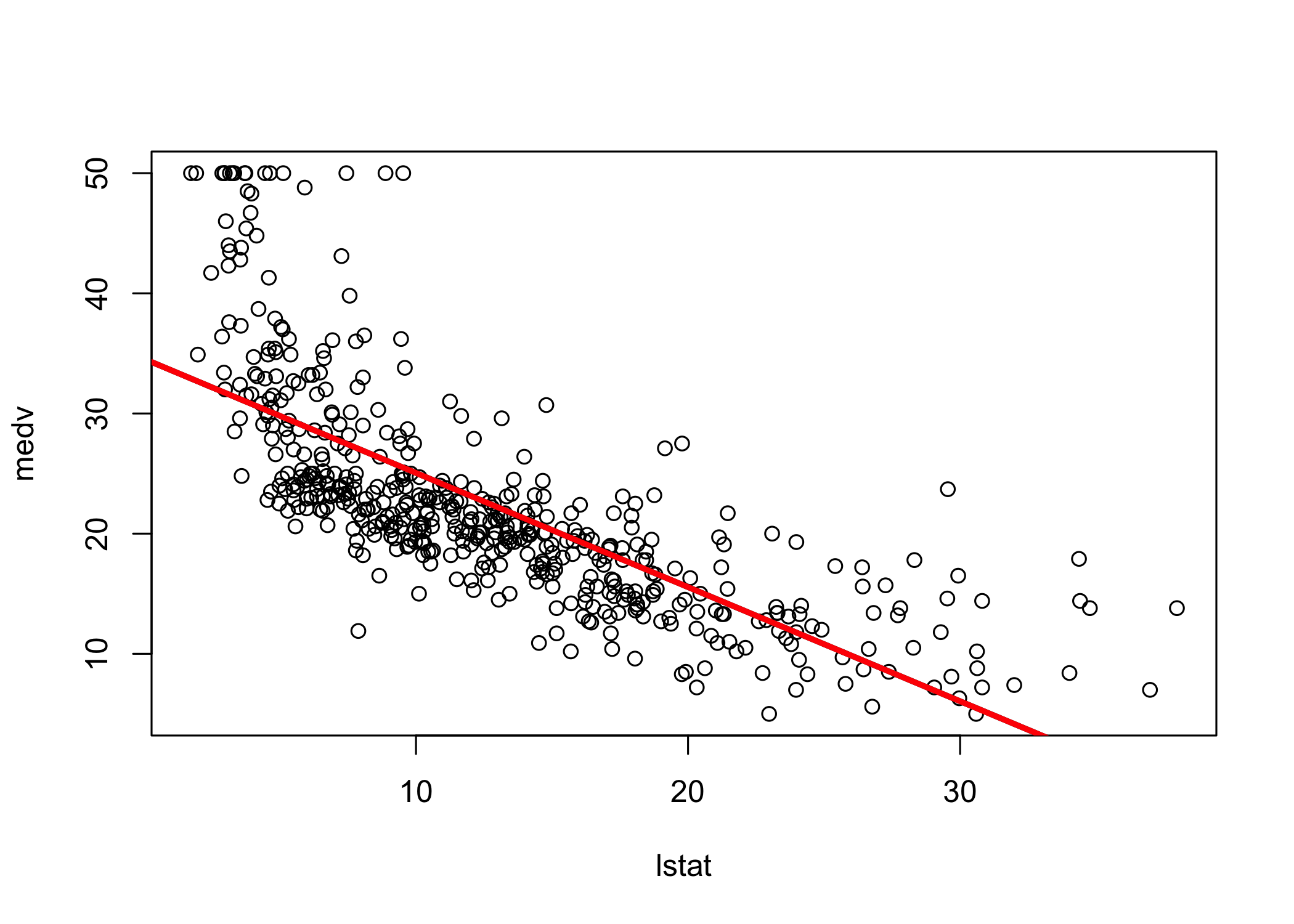
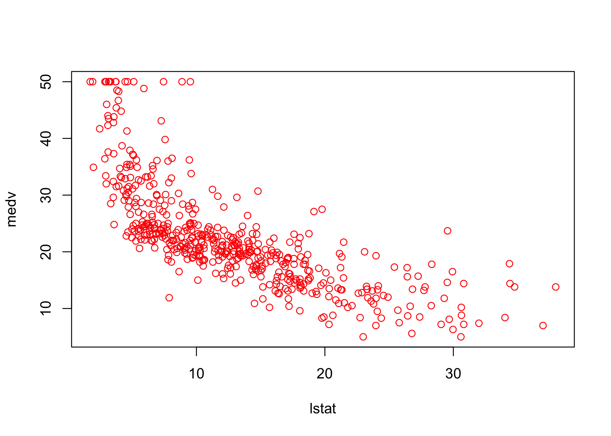
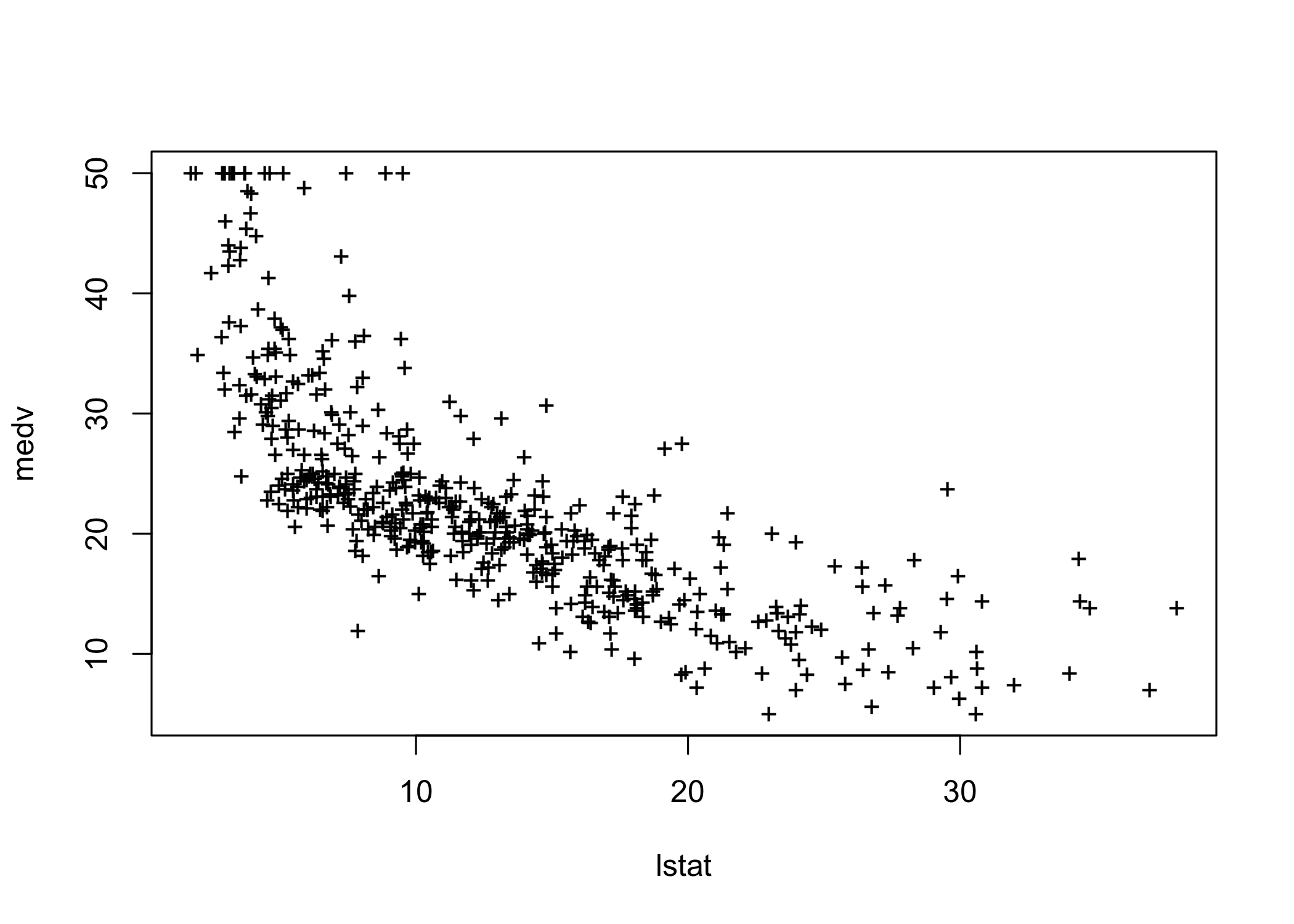
  • slope = b

• Plot options:

  • lwd controls line width
  • col controls color
  • pch controls plotting symbol

plot(lstat, medv)
abline(lm.fit, lwd = 3)
abline(lm.fit, lwd = 3, col = "red")

plot(lstat, medv, col = "red")

plot(lstat, medv, pch = 20)

plot(lstat, medv, pch = "+")

plot(1:20, 1:20, pch = 1:20)

Non-linear Transformations of the Predictors

• lm() can include transformed predictors
  
• Use I() when arithmetic operators would otherwise be interpreted specially in a formula
  
• Example: I(lstat^2) adds a quadratic term

lm.fit2 <- lm(medv ~ lstat + I(lstat^2), data = Boston)
summary(lm.fit2)

Call:
lm(formula = medv ~ lstat + I(lstat^2), data = Boston)

Residuals:
     Min       1Q   Median       3Q      Max 
-15.2834  -3.8313  -0.5295   2.3095  25.4148 

Coefficients:
             Estimate Std. Error t value Pr(>|t|)    
(Intercept) 42.862007   0.872084   49.15   <2e-16 ***
lstat       -2.332821   0.123803  -18.84   <2e-16 ***
I(lstat^2)   0.043547   0.003745   11.63   <2e-16 ***
---
Signif. codes:  0 '***' 0.001 '**' 0.01 '*' 0.05 '.' 0.1 ' ' 1

Residual standard error: 5.524 on 503 degrees of freedom
Multiple R-squared:  0.6407,    Adjusted R-squared:  0.6393 
F-statistic: 448.5 on 2 and 503 DF,  p-value: < 2.2e-16

• The quadratic term appears to improve the model
  
• Compare the linear and quadratic models with anova()

lm.fit <- lm(medv ~ lstat, data = Boston)
anova(lm.fit, lm.fit2)

Analysis of Variance Table

Model 1: medv ~ lstat
Model 2: medv ~ lstat + I(lstat^2)
  Res.Df   RSS Df Sum of Sq     F    Pr(>F)    
1    504 19472                                 
2    503 15347  1    4125.1 135.2 < 2.2e-16 ***
---
Signif. codes:  0 '***' 0.001 '**' 0.01 '*' 0.05 '.' 0.1 ' ' 1

• Model 1: linear fit with lstat
  

• Model 2: quadratic fit with lstat and lstat^2
  

• anova() tests whether the larger model improves fit significantly
  

• Very small p-value indicates strong evidence in favor of the quadratic model

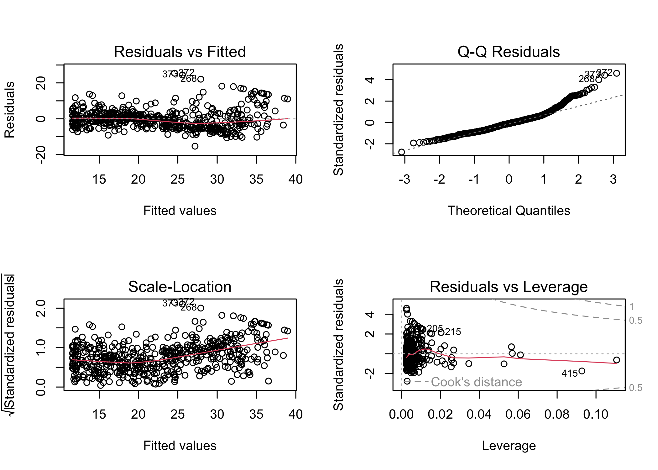
• Check the residual diagnostics for the quadratic model

par(mfrow = c(2, 2))
plot(lm.fit2)

• With the quadratic term included, residual patterns are reduced

• For higher-order polynomials, poly() is more convenient than writing each power manually
  

• Example: fifth-order polynomial fit

lm.fit5 <- lm(medv ~ poly(lstat, 5), data = Boston)
summary(lm.fit5)

Call:
lm(formula = medv ~ poly(lstat, 5), data = Boston)

Residuals:
     Min       1Q   Median       3Q      Max 
-13.5433  -3.1039  -0.7052   2.0844  27.1153 

Coefficients:
                 Estimate Std. Error t value Pr(>|t|)    
(Intercept)       22.5328     0.2318  97.197  < 2e-16 ***
poly(lstat, 5)1 -152.4595     5.2148 -29.236  < 2e-16 ***
poly(lstat, 5)2   64.2272     5.2148  12.316  < 2e-16 ***
poly(lstat, 5)3  -27.0511     5.2148  -5.187 3.10e-07 ***
poly(lstat, 5)4   25.4517     5.2148   4.881 1.42e-06 ***
poly(lstat, 5)5  -19.2524     5.2148  -3.692 0.000247 ***
---
Signif. codes:  0 '***' 0.001 '**' 0.01 '*' 0.05 '.' 0.1 ' ' 1

Residual standard error: 5.215 on 500 degrees of freedom
Multiple R-squared:  0.6817,    Adjusted R-squared:  0.6785 
F-statistic: 214.2 on 5 and 500 DF,  p-value: < 2.2e-16

• Higher-order polynomial terms can improve fit
  

• In this example, terms beyond fifth order are not significant

• By default, poly() uses orthogonal polynomials
  

• These are not the raw powers of the predictor
  

• Fitted values are the same as with raw polynomials, but coefficients differ
  

• Use raw = TRUE if raw powers are desired

• We are not restricted to polynomial transformations
  

• Example: log transformation

summary(lm(medv ~ log(rm), data = Boston))

Call:
lm(formula = medv ~ log(rm), data = Boston)

Residuals:
    Min      1Q  Median      3Q     Max 
-19.487  -2.875  -0.104   2.837  39.816 

Coefficients:
            Estimate Std. Error t value Pr(>|t|)    
(Intercept)  -76.488      5.028  -15.21   <2e-16 ***
log(rm)       54.055      2.739   19.73   <2e-16 ***
---
Signif. codes:  0 '***' 0.001 '**' 0.01 '*' 0.05 '.' 0.1 ' ' 1

Residual standard error: 6.915 on 504 degrees of freedom
Multiple R-squared:  0.4358,    Adjusted R-squared:  0.4347 
F-statistic: 389.3 on 1 and 504 DF,  p-value: < 2.2e-16

Cross-Validation

• In this lab, we explore resampling methods
  
• Focus:
  • validation set approach
  • leave-one-out cross-validation (LOOCV)
  • k-fold cross-validation
    
• Some commands may take a while to run

The Validation Set Approach

• Use the validation set approach to estimate test error
  
• Work with the Auto data set
  
• Set a random seed for reproducibility
  
• This ensures the same training/validation split each time

library(ISLR2)
set.seed(1)
train <- sample(392, 196)

• Split the data into two halves
  
• Here, train contains the indices of the training observations
  
• Fit the model only on the training set using subset = train

lm.fit <- lm(mpg ~ horsepower, data = Auto, subset = train)

• Use predict() to compute fitted values for all observations
  
• Compute validation MSE on the observations not in the training set
  
• -train selects the validation observations

attach(Auto)
mean((mpg - predict(lm.fit, Auto))[-train]^2)

[1] 23.26601

• Estimate test MSE for quadratic and cubic models
  
• Use poly() to fit polynomial regressions

lm.fit2 <- lm(mpg ~ poly(horsepower, 2), data = Auto, 
    subset = train)
mean((mpg - predict(lm.fit2, Auto))[-train]^2)

[1] 18.71646

lm.fit3 <- lm(mpg ~ poly(horsepower, 3), data = Auto, 
    subset = train)
mean((mpg - predict(lm.fit3, Auto))[-train]^2)

[1] 18.79401

• Different training/validation splits give slightly different results
  
• Repeat with a different random seed

set.seed(2)
train <- sample(392, 196)
lm.fit <- lm(mpg ~ horsepower, subset = train)
mean((mpg - predict(lm.fit, Auto))[-train]^2)

[1] 25.72651

lm.fit2 <- lm(mpg ~ poly(horsepower, 2), data = Auto, 
    subset = train)
mean((mpg - predict(lm.fit2, Auto))[-train]^2)

[1] 20.43036

lm.fit3 <- lm(mpg ~ poly(horsepower, 3), data = Auto, 
    subset = train)
mean((mpg - predict(lm.fit3, Auto))[-train]^2)

[1] 20.38533

• Main result:
  • quadratic model improves over linear
  • little evidence that cubic improves further

Leave-One-Out Cross-Validation

• LOOCV can be computed with cv.glm()
  
• cv.glm() works with models fit using glm()
  
• Without a family argument, glm() performs linear regression
  
• So glm() and lm() give the same fit here

glm.fit <- glm(mpg ~ horsepower, data = Auto)
coef(glm.fit)

(Intercept)  horsepower 
 39.9358610  -0.1578447 

lm.fit <- lm(mpg ~ horsepower, data = Auto)
coef(lm.fit)

(Intercept)  horsepower 
 39.9358610  -0.1578447 

• Use glm() because it works with cv.glm()
  
• cv.glm() is in the boot package

library(boot)
glm.fit <- glm(mpg ~ horsepower, data = Auto)
cv.err <- cv.glm(Auto, glm.fit)
cv.err$delta

[1] 24.23151 24.23114

• cv.glm() returns a list
  

• delta contains the cross-validation estimates
  

• For LOOCV, the two values are essentially the same

• Compute LOOCV error for polynomial models of degree 1 to 10
  

• Store the results in a vector

cv.error <- rep(0, 10)
for (i in 1:10) {
  glm.fit <- glm(mpg ~ poly(horsepower, i), data = Auto)
  cv.error[i] <- cv.glm(Auto, glm.fit)$delta[1]
}
cv.error

 [1] 24.23151 19.24821 19.33498 19.42443 19.03321 18.97864 18.83305 18.96115
 [9] 19.06863 19.49093

• Main pattern:
  • large drop from linear to quadratic
  • little improvement beyond degree 2

k-Fold Cross-Validation

• cv.glm() can also perform k-fold CV
  
• Here we use:
  • k = 10
• Again evaluate polynomial models of degree 1 to 10

set.seed(17)
cv.error.10 <- rep(0, 10)
for (i in 1:10) {
  glm.fit <- glm(mpg ~ poly(horsepower, i), data = Auto)
  cv.error.10[i] <- cv.glm(Auto, glm.fit, K = 10)$delta[1]
}
cv.error.10

 [1] 24.27207 19.26909 19.34805 19.29496 19.03198 18.89781 19.12061 19.14666
 [9] 18.87013 20.95520

• k-fold CV is faster to compute than LOOCV here
  
• Results are similar:
  • quadratic model improves over linear
  • higher-order terms add little
• With LOOCV, the two values in delta are almost identical
  
• With k-fold CV, they differ slightly:
  • first value = standard k-fold CV estimate
  • second value = bias-corrected estimate
    
• On this data set, the difference is very small