Lab 4
Decision Trees, Bagging, Random Forests, and Boosting
Fitting Classification Trees
- The
treelibrary in R is used to construct regression trees
- Fit a regression tree using the
Bostondataset
- Split data into a training set
- Train the tree model on the training data
library(MASS)
set.seed(1)
train <- sample(1:nrow(Boston), nrow(Boston) / 2)
tree.boston <- tree(medv ~ ., Boston, subset = train)
summary(tree.boston)
Regression tree:
tree(formula = medv ~ ., data = Boston, subset = train)
Variables actually used in tree construction:
[1] "rm"    "lstat" "crim"  "age"
Number of terminal nodes:  7
Residual mean deviance:  10.38 = 2555 / 246
Distribution of residuals:
    Min.  1st Qu.   Median     Mean  3rd Qu.     Max.
-10.1800 -1.7770 -0.1775 0.0000 1.9230 16.5800 summary()shows only 4 variables are used in the tree
- In regression trees, deviance = sum of squared errors (SSE)
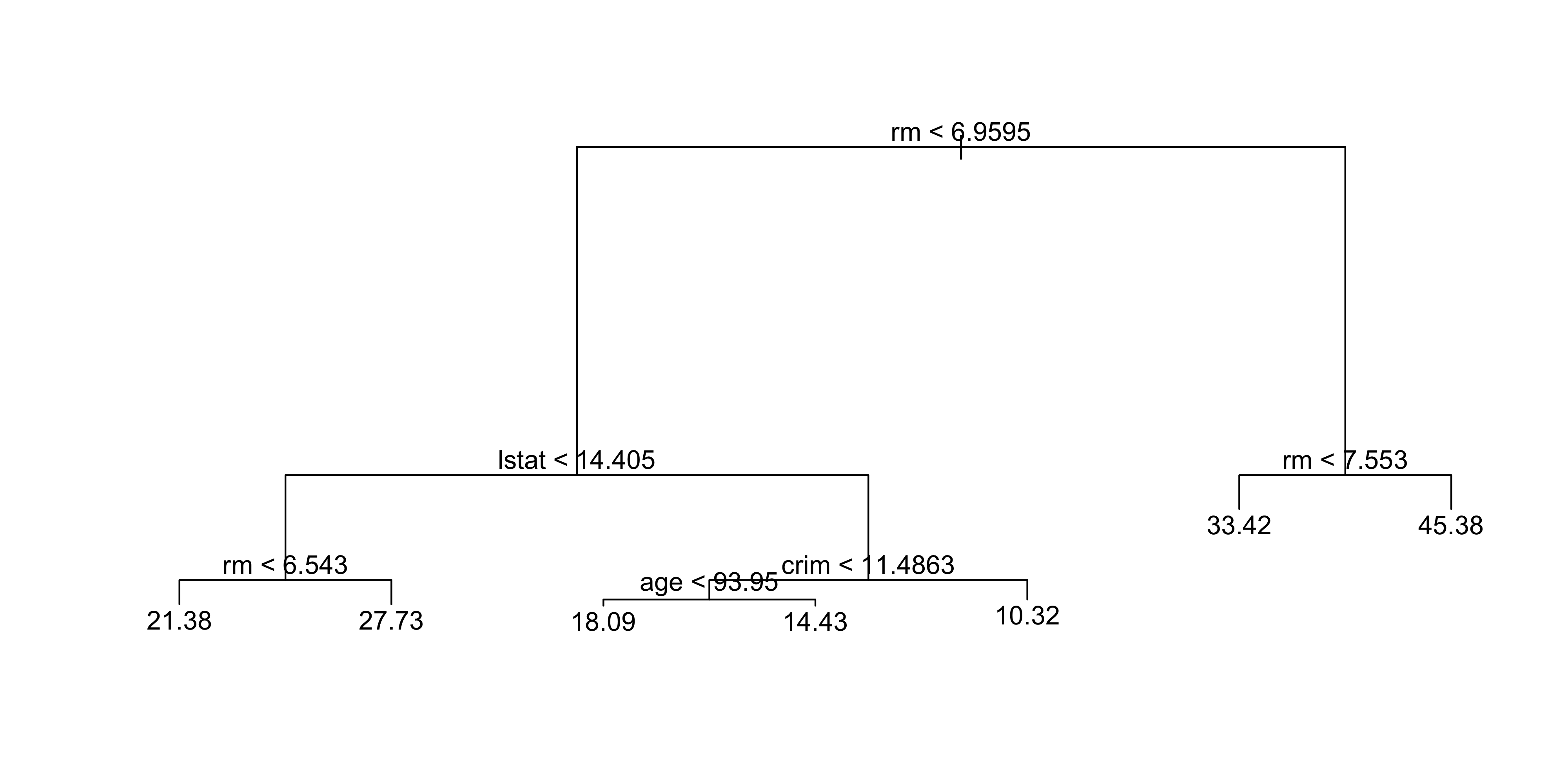
lstat: % of lower socioeconomic status
rm: average number of roomsInterpretation:
- Higher
rm→ higher house prices
- Lower
lstat→ higher house prices
- Example:
rm ≥ 7.553→ predicted price ≈ $45,400
- Higher
Model flexibility:
- Larger tree can be grown using
tree.control(..., mindev = 0)
- Larger tree can be grown using
Next step:
- Use
cv.tree()to evaluate pruning via cross-validation
- Use
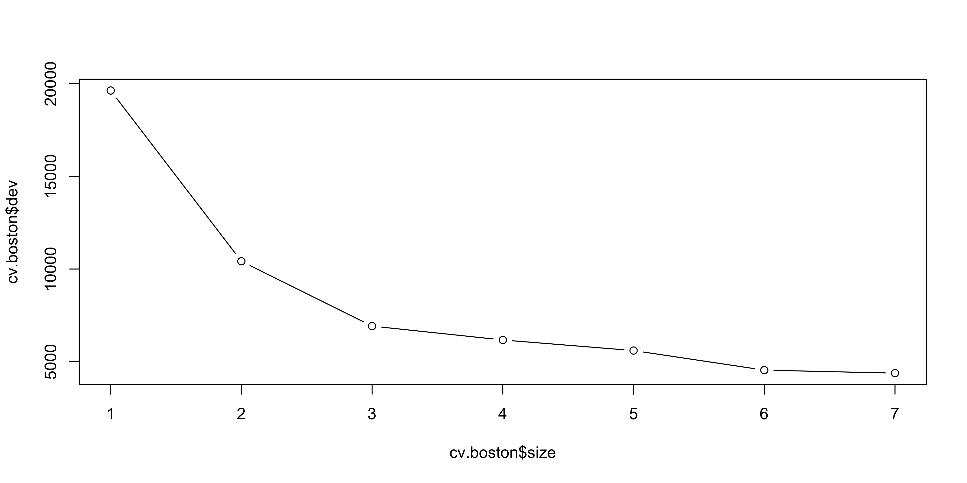
- Cross-validation selects the most complex tree in this case
- Tree can still be pruned manually if desired
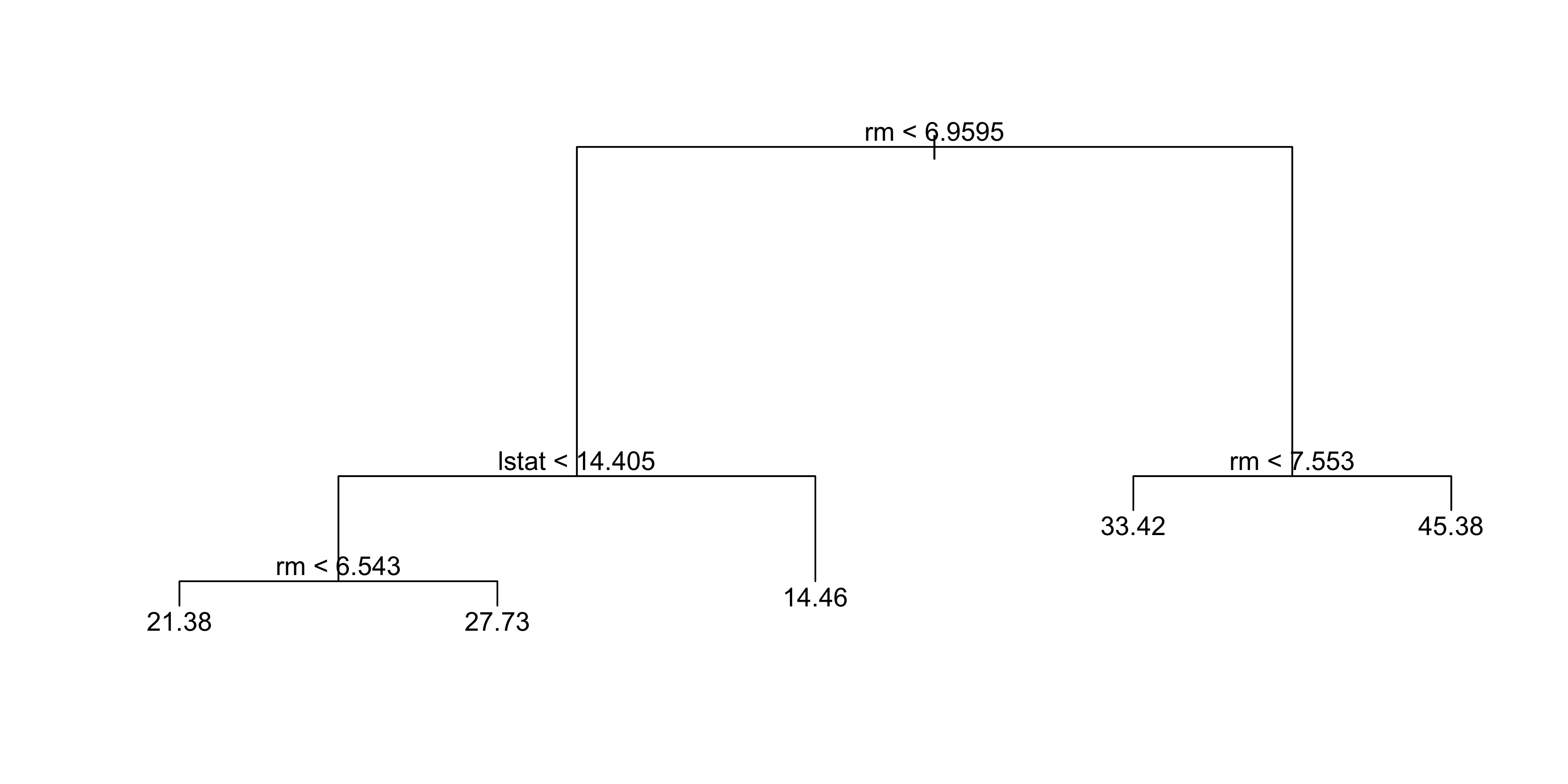
- Based on cross-validation, the unpruned tree is selected
- Use the unpruned tree to make predictions on the test set
yhat <- predict(tree.boston, newdata = Boston[-train, ])
boston.test <- Boston[-train, "medv"]
plot(yhat, boston.test)
abline(0, 1)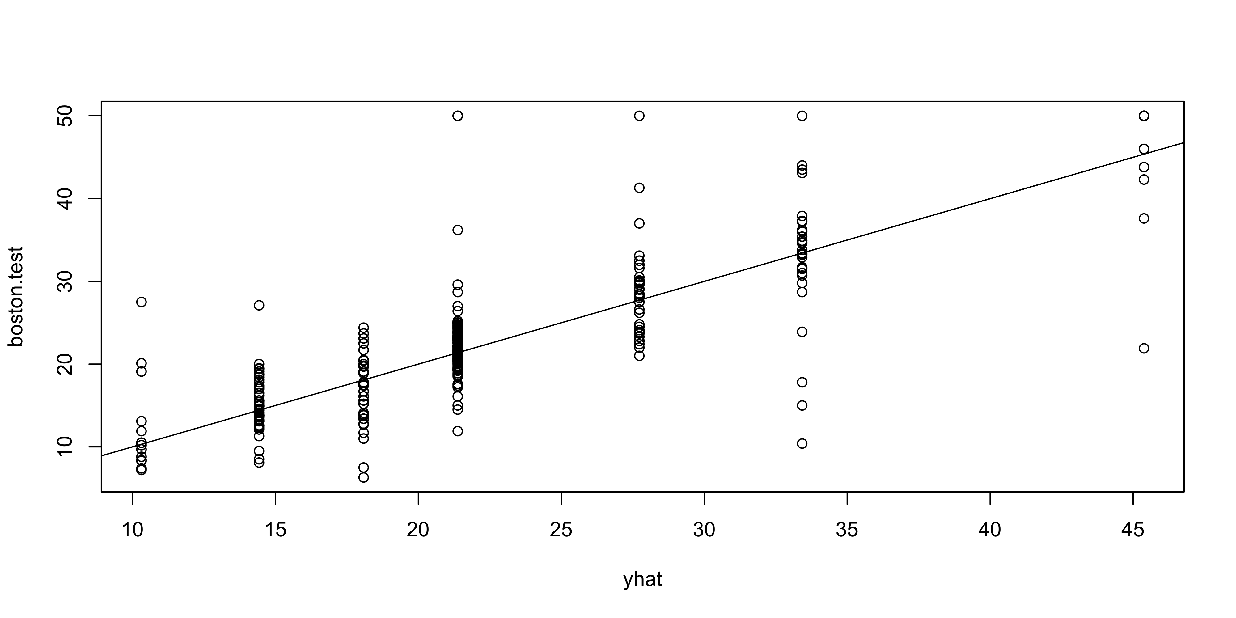
[1] 35.28688- Test set MSE ≈ 35.29
- RMSE ≈ 5.941
- Predictions are on average within ~$5,941 of true median house values
Bagging and Random Forests
- Apply bagging and random forests using the
randomForestpackage in R
- Bagging = special case of random forest with m = p (all predictors used at each split)
library(randomForest)
set.seed(1)
bag.boston <- randomForest(medv ~ ., data = Boston,
    subset = train, mtry = 12, importance = TRUE)
bag.boston
Call:
 randomForest(formula = medv ~ ., data = Boston, mtry = 12, importance = TRUE,      subset = train)
               Type of random forest: regression
                     Number of trees: 500
No. of variables tried at each split: 12

          Mean of squared residuals: 11.10176
                    % Var explained: 85.56
mtry = 12→ all 12 predictors used at each split
- This corresponds to bagging
- Evaluate model performance on the test set
yhat.bag <- predict(bag.boston, newdata = Boston[-train, ])
plot(yhat.bag, boston.test)
abline(0, 1)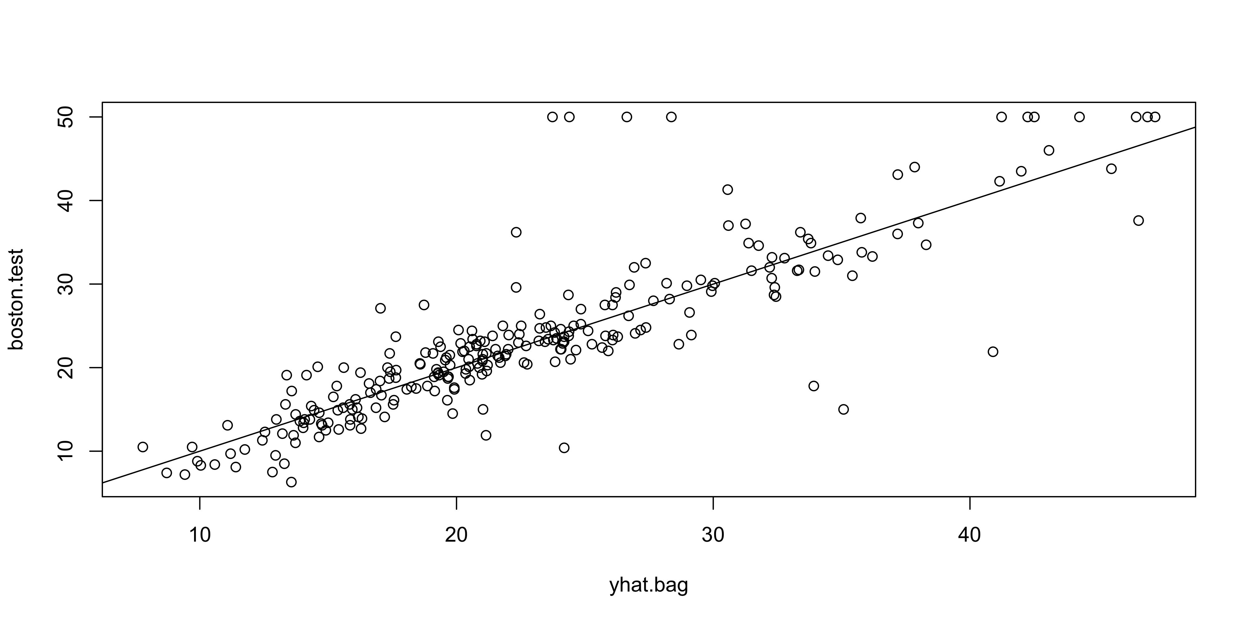
[1] 23.38773- Bagged model test MSE ≈ 23.42
- Significantly lower than single tree (~2/3 of its error)
- Number of trees can be controlled with the
ntreeparameter
bag.boston <- randomForest(medv ~ ., data = Boston,
    subset = train, mtry = 12, ntree = 25)
yhat.bag <- predict(bag.boston, newdata = Boston[-train, ])
mean((yhat.bag - boston.test)^2)
[1] 25.19144- Random forests are built like bagging but with smaller
mtry
- Default
mtry:- Regression: p/3
- Here,
mtry = 6is used
set.seed(1)
rf.boston <- randomForest(medv ~ ., data = Boston,
    subset = train, mtry = 6, importance = TRUE)
yhat.rf <- predict(rf.boston, newdata = Boston[-train, ])
mean((yhat.rf - boston.test)^2)
[1] 19.62021- Random forest test MSE ≈ 20.07
- Improves over bagging performance
- Use
importance()to evaluate variable importance
          %IncMSE IncNodePurity
crim    16.697017    1076.08786
zn       3.625784      88.35342
indus    4.968621     609.53356
chas     1.061432      52.21793
nox     13.518179     709.87339
rm      32.343305    7857.65451
age     13.272498     612.21424
dis      9.032477     714.94674
rad      2.878434      95.80598
tax      9.118801     364.92479
ptratio  8.467062     823.93341
black    7.579482     275.62272
lstat 27.129817 6027.63740- Two measures of variable importance:
- Mean decrease in accuracy (via permutation on out-of-bag samples)
- Mean decrease in node impurity (averaged over all trees)
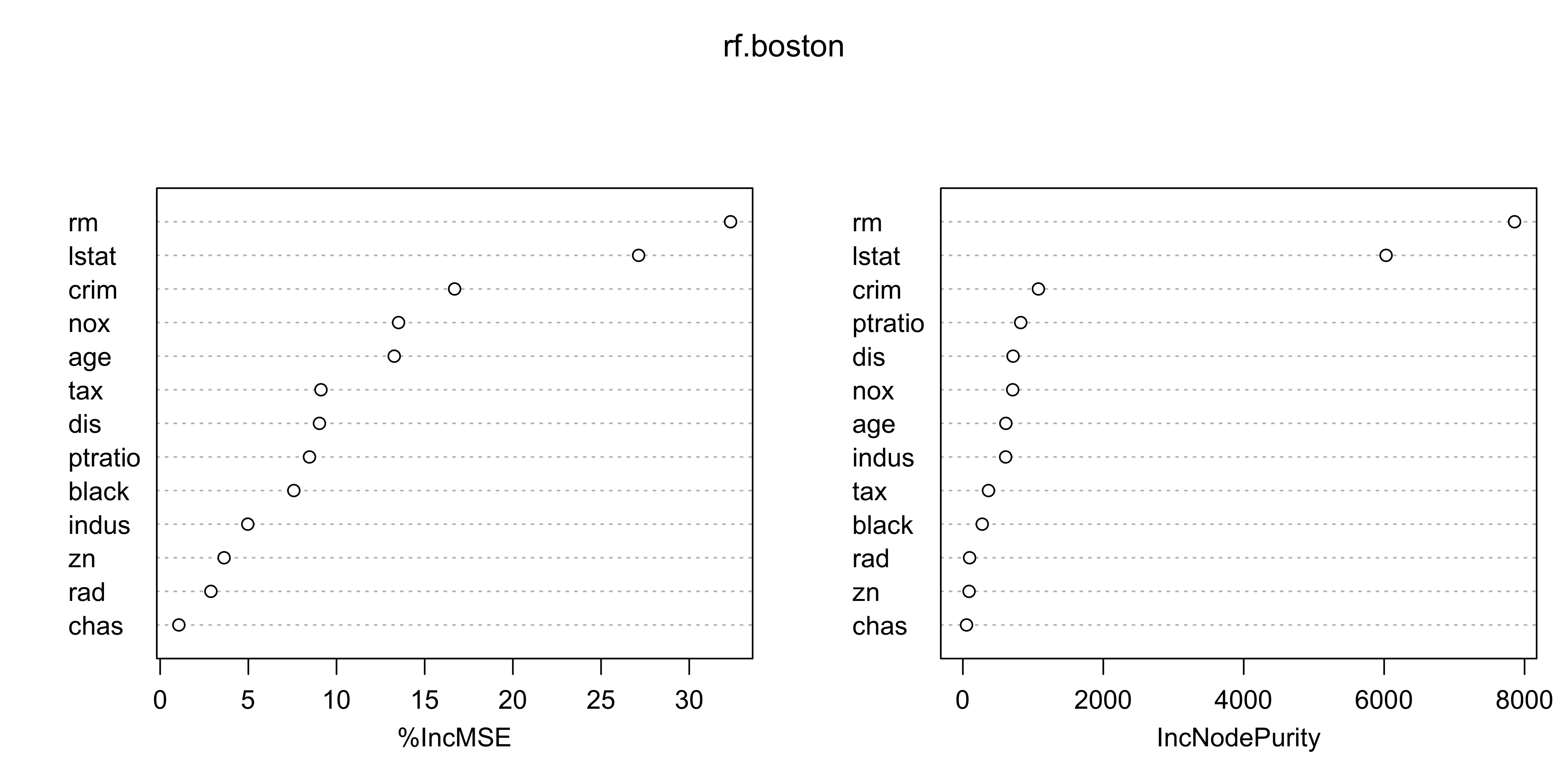
- Most important variables in the random forest:
lstat(wealth / socioeconomic status)
rm(house size / number of rooms)
Boosting
- Use the
gbmpackage to fit boosted regression trees
- Apply
gbm()to theBostondataset
- Set
distribution = "gaussian"for regression problems
summary()provides:- Relative influence plot
- Numerical measures of variable importance
- Relative influence plot
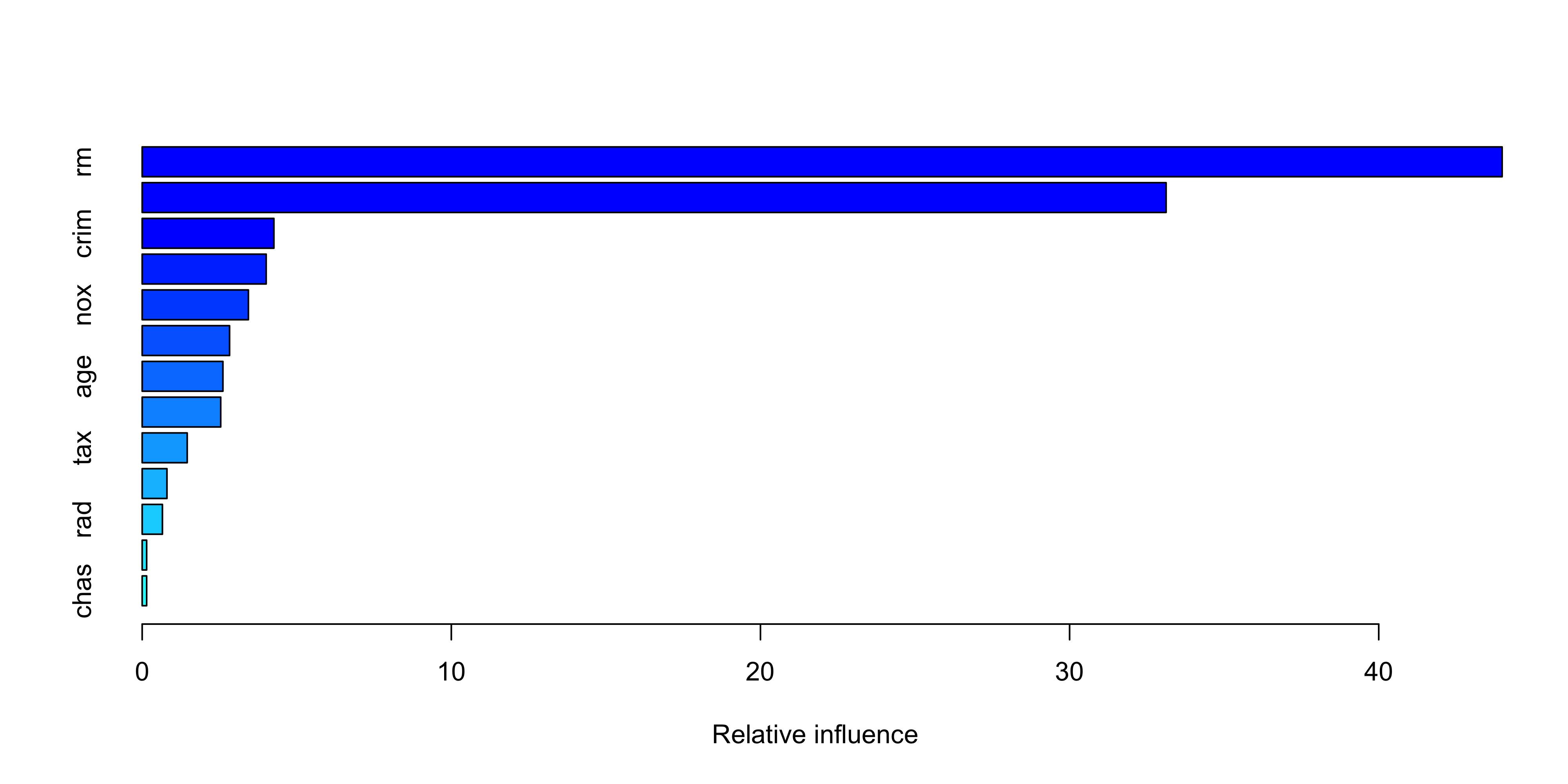
            var    rel.inf
rm           rm 43.9919329
lstat     lstat 33.1216941
crim       crim  4.2604167
dis         dis  4.0111090
nox         nox  3.4353017
black     black  2.8267554
age         age  2.6113938
ptratio ptratio  2.5403035
tax         tax  1.4565654
indus     indus  0.8008740
rad         rad  0.6546400
zn           zn  0.1446149
chas chas 0.1443986lstatandrmare the most important variables
- Partial dependence plots can be generated for these variables
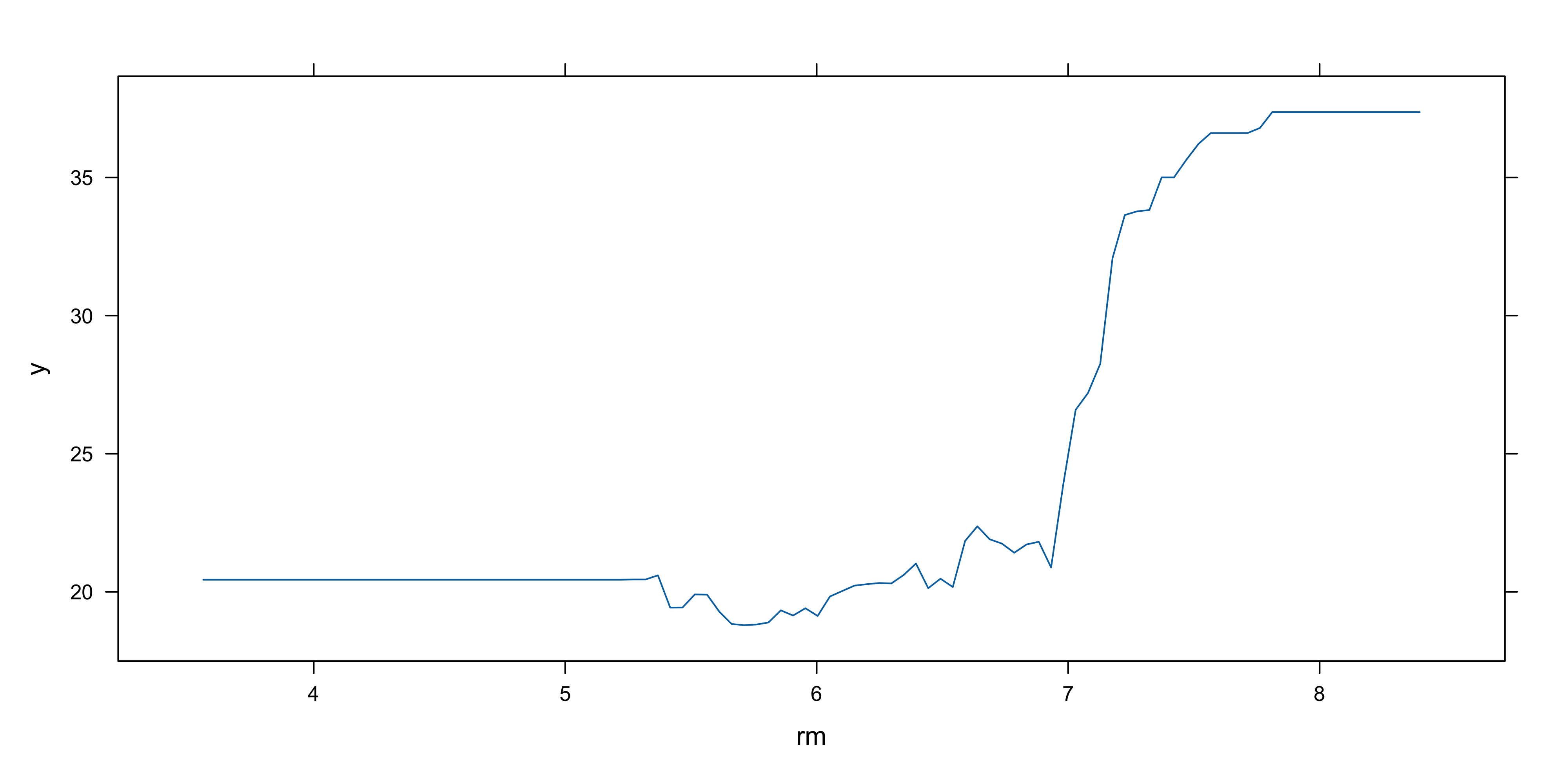
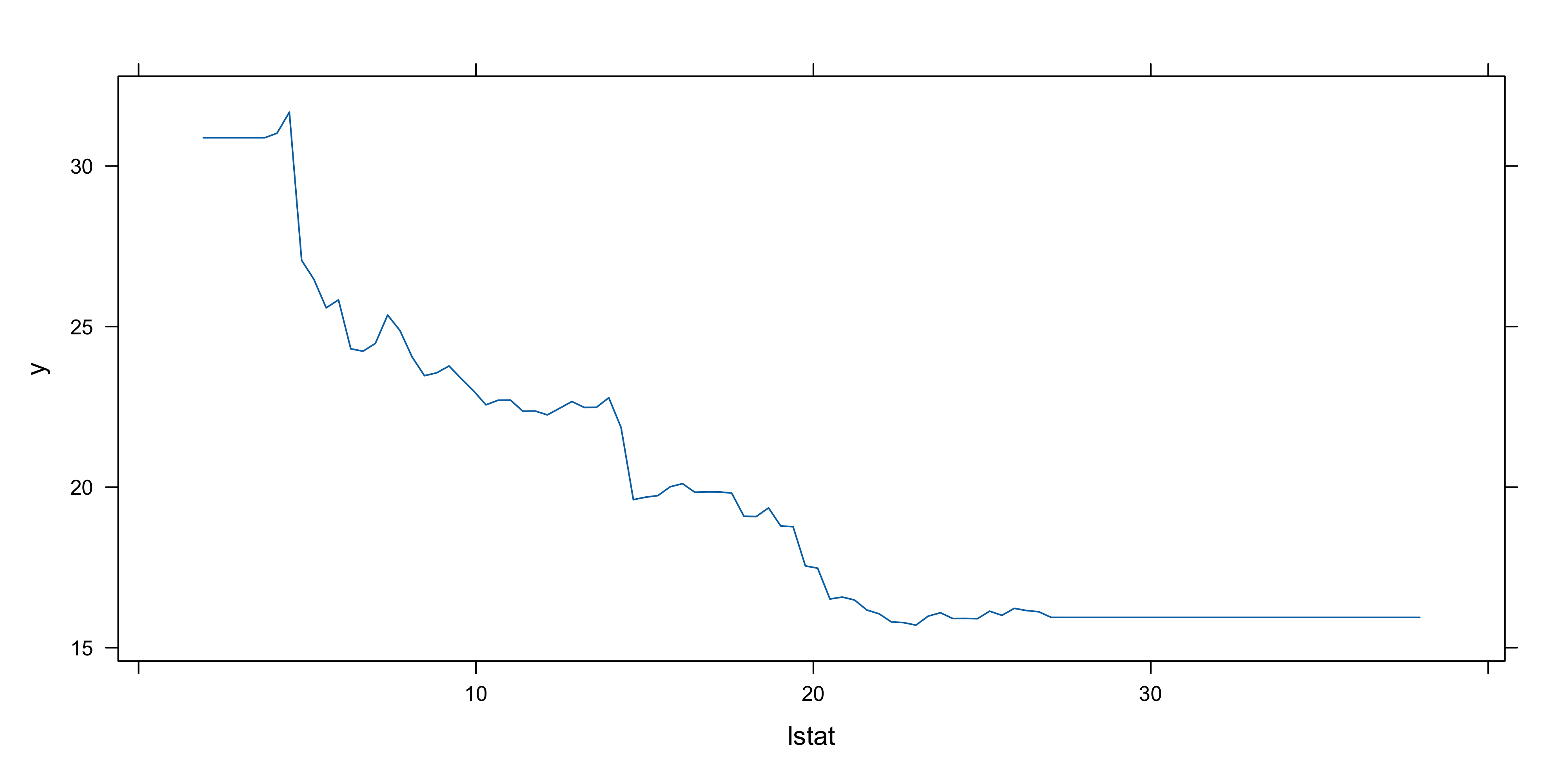
- Partial dependence plots show marginal effect of variables on response
- Effects observed:
- Higher
rm→ higher house prices
- Higher
lstat→ lower house prices
- Higher
- Use boosted model to predict
medvon the test set
yhat.boost <- predict(boost.boston,
    newdata = Boston[-train, ], n.trees = 5000)
mean((yhat.boost - boston.test)^2)
[1] 18.84709- Boosting test MSE ≈ 18.39
- Outperforms random forests and bagging
- Model can be tuned via shrinkage parameter \lambda
- Example: use \lambda = 0.2
boost.boston <- gbm(medv ~ ., data = Boston[train, ],
    distribution = "gaussian", n.trees = 5000,
    interaction.depth = 4, shrinkage = 0.2, verbose = FALSE)
yhat.boost <- predict(boost.boston,
    newdata = Boston[-train, ], n.trees = 5000)
mean((yhat.boost - boston.test)^2)
[1] 18.33455- Using \lambda = 0.2 results in lower test MSE than \lambda = 0.001