Lab 3

Introduction to Statistical Learning - PISE

Author

Affiliation

Aldo Solari

Ca’ Foscari University of Venice

Linear Regression

Multiple Linear Regression

• Fit multiple regression models with the lm() function
  
• Syntax: lm(y ~ x1 + x2 + x3, data = ...)

library(MASS)
lm.fit <- lm(medv ~ lstat + age, data = Boston)
summary(lm.fit)

Call:
lm(formula = medv ~ lstat + age, data = Boston)

Residuals:
    Min      1Q  Median      3Q     Max 
-15.981  -3.978  -1.283   1.968  23.158 

Coefficients:
            Estimate Std. Error t value Pr(>|t|)    
(Intercept) 33.22276    0.73085  45.458  < 2e-16 ***
lstat       -1.03207    0.04819 -21.416  < 2e-16 ***
age          0.03454    0.01223   2.826  0.00491 ** 
---
Signif. codes:  0 '***' 0.001 '**' 0.01 '*' 0.05 '.' 0.1 ' ' 1

Residual standard error: 6.173 on 503 degrees of freedom
Multiple R-squared:  0.5513,    Adjusted R-squared:  0.5495 
F-statistic:   309 on 2 and 503 DF,  p-value: < 2.2e-16

• To use all predictors, write . as shorthand

lm.fit <- lm(medv ~ ., data = Boston)
summary(lm.fit)

Call:
lm(formula = medv ~ ., data = Boston)

Residuals:
    Min      1Q  Median      3Q     Max 
-15.595  -2.730  -0.518   1.777  26.199 

Coefficients:
              Estimate Std. Error t value Pr(>|t|)    
(Intercept)  3.646e+01  5.103e+00   7.144 3.28e-12 ***
crim        -1.080e-01  3.286e-02  -3.287 0.001087 ** 
zn           4.642e-02  1.373e-02   3.382 0.000778 ***
indus        2.056e-02  6.150e-02   0.334 0.738288    
chas         2.687e+00  8.616e-01   3.118 0.001925 ** 
nox         -1.777e+01  3.820e+00  -4.651 4.25e-06 ***
rm           3.810e+00  4.179e-01   9.116  < 2e-16 ***
age          6.922e-04  1.321e-02   0.052 0.958229    
dis         -1.476e+00  1.995e-01  -7.398 6.01e-13 ***
rad          3.060e-01  6.635e-02   4.613 5.07e-06 ***
tax         -1.233e-02  3.760e-03  -3.280 0.001112 ** 
ptratio     -9.527e-01  1.308e-01  -7.283 1.31e-12 ***
black        9.312e-03  2.686e-03   3.467 0.000573 ***
lstat       -5.248e-01  5.072e-02 -10.347  < 2e-16 ***
---
Signif. codes:  0 '***' 0.001 '**' 0.01 '*' 0.05 '.' 0.1 ' ' 1

Residual standard error: 4.745 on 492 degrees of freedom
Multiple R-squared:  0.7406,    Adjusted R-squared:  0.7338 
F-statistic: 108.1 on 13 and 492 DF,  p-value: < 2.2e-16

• Components of the summary object can be extracted by name
  
• Examples:
  • summary(lm.fit)$r.sq
  • summary(lm.fit)$sigma
• vif() from the car package computes variance inflation factors
  
• VIFs help assess multicollinearity

library(car)

Loading required package: carData

vif(lm.fit)

    crim       zn    indus     chas      nox       rm      age      dis 
1.792192 2.298758 3.991596 1.073995 4.393720 1.933744 3.100826 3.955945 
     rad      tax  ptratio    black    lstat 
7.484496 9.008554 1.799084 1.348521 2.941491 

• Exclude one predictor using - in the formula
  
• Example: remove age

lm.fit1 <- lm(medv ~ . - age, data = Boston)
summary(lm.fit1)

Call:
lm(formula = medv ~ . - age, data = Boston)

Residuals:
     Min       1Q   Median       3Q      Max 
-15.6054  -2.7313  -0.5188   1.7601  26.2243 

Coefficients:
              Estimate Std. Error t value Pr(>|t|)    
(Intercept)  36.436927   5.080119   7.172 2.72e-12 ***
crim         -0.108006   0.032832  -3.290 0.001075 ** 
zn            0.046334   0.013613   3.404 0.000719 ***
indus         0.020562   0.061433   0.335 0.737989    
chas          2.689026   0.859598   3.128 0.001863 ** 
nox         -17.713540   3.679308  -4.814 1.97e-06 ***
rm            3.814394   0.408480   9.338  < 2e-16 ***
dis          -1.478612   0.190611  -7.757 5.03e-14 ***
rad           0.305786   0.066089   4.627 4.75e-06 ***
tax          -0.012329   0.003755  -3.283 0.001099 ** 
ptratio      -0.952211   0.130294  -7.308 1.10e-12 ***
black         0.009321   0.002678   3.481 0.000544 ***
lstat        -0.523852   0.047625 -10.999  < 2e-16 ***
---
Signif. codes:  0 '***' 0.001 '**' 0.01 '*' 0.05 '.' 0.1 ' ' 1

Residual standard error: 4.74 on 493 degrees of freedom
Multiple R-squared:  0.7406,    Adjusted R-squared:  0.7343 
F-statistic: 117.3 on 12 and 493 DF,  p-value: < 2.2e-16

• Alternatively, update an existing model with update()

lm.fit1 <- update(lm.fit, ~ . - age)

Interaction Terms

• Include interaction terms with :
  
• Example: lstat:age
  
• Use * as shorthand for:
  • main effects
  • interaction term
• lstat * age is shorthand for:
  • lstat + age + lstat:age

summary(lm(medv ~ lstat * age, data = Boston))

Call:
lm(formula = medv ~ lstat * age, data = Boston)

Residuals:
    Min      1Q  Median      3Q     Max 
-15.806  -4.045  -1.333   2.085  27.552 

Coefficients:
              Estimate Std. Error t value Pr(>|t|)    
(Intercept) 36.0885359  1.4698355  24.553  < 2e-16 ***
lstat       -1.3921168  0.1674555  -8.313 8.78e-16 ***
age         -0.0007209  0.0198792  -0.036   0.9711    
lstat:age    0.0041560  0.0018518   2.244   0.0252 *  
---
Signif. codes:  0 '***' 0.001 '**' 0.01 '*' 0.05 '.' 0.1 ' ' 1

Residual standard error: 6.149 on 502 degrees of freedom
Multiple R-squared:  0.5557,    Adjusted R-squared:  0.5531 
F-statistic: 209.3 on 3 and 502 DF,  p-value: < 2.2e-16

Qualitative Predictors

• Carseats is another dataset in ISLR2
  
• Response variable: Sales
  
• Predictors include both quantitative and qualitative variables

library(ISLR2)

Attaching package: 'ISLR2'

The following object is masked from 'package:MASS':

    Boston

head(Carseats)

  Sales CompPrice Income Advertising Population Price ShelveLoc Age Education
1  9.50       138     73          11        276   120       Bad  42        17
2 11.22       111     48          16        260    83      Good  65        10
3 10.06       113     35          10        269    80    Medium  59        12
4  7.40       117    100           4        466    97    Medium  55        14
5  4.15       141     64           3        340   128       Bad  38        13
6 10.81       124    113          13        501    72       Bad  78        16
  Urban  US
1   Yes Yes
2   Yes Yes
3   Yes Yes
4   Yes Yes
5   Yes  No
6    No Yes

• ShelveLoc is a qualitative predictor
  
• Levels:
  • Bad
  • Medium
  • Good
• R automatically creates dummy variables for qualitative predictors

lm.fit <- lm(Sales ~ . + Income:Advertising + Price:Age, 
    data = Carseats)
summary(lm.fit)

Call:
lm(formula = Sales ~ . + Income:Advertising + Price:Age, data = Carseats)

Residuals:
    Min      1Q  Median      3Q     Max 
-2.9208 -0.7503  0.0177  0.6754  3.3413 

Coefficients:
                     Estimate Std. Error t value Pr(>|t|)    
(Intercept)         6.5755654  1.0087470   6.519 2.22e-10 ***
CompPrice           0.0929371  0.0041183  22.567  < 2e-16 ***
Income              0.0108940  0.0026044   4.183 3.57e-05 ***
Advertising         0.0702462  0.0226091   3.107 0.002030 ** 
Population          0.0001592  0.0003679   0.433 0.665330    
Price              -0.1008064  0.0074399 -13.549  < 2e-16 ***
ShelveLocGood       4.8486762  0.1528378  31.724  < 2e-16 ***
ShelveLocMedium     1.9532620  0.1257682  15.531  < 2e-16 ***
Age                -0.0579466  0.0159506  -3.633 0.000318 ***
Education          -0.0208525  0.0196131  -1.063 0.288361    
UrbanYes            0.1401597  0.1124019   1.247 0.213171    
USYes              -0.1575571  0.1489234  -1.058 0.290729    
Income:Advertising  0.0007510  0.0002784   2.698 0.007290 ** 
Price:Age           0.0001068  0.0001333   0.801 0.423812    
---
Signif. codes:  0 '***' 0.001 '**' 0.01 '*' 0.05 '.' 0.1 ' ' 1

Residual standard error: 1.011 on 386 degrees of freedom
Multiple R-squared:  0.8761,    Adjusted R-squared:  0.8719 
F-statistic:   210 on 13 and 386 DF,  p-value: < 2.2e-16

• Use contrasts() to see the dummy-variable coding used by R

attach(Carseats)
contrasts(ShelveLoc)

       Good Medium
Bad       0      0
Good      1      0
Medium    0      1

• Use ?contrasts for more information

• Here:

  • ShelveLocGood = 1 if location is good, 0 otherwise
  • ShelveLocMedium = 1 if location is medium, 0 otherwise
  • Bad is the baseline category

• Positive coefficients indicate higher sales relative to the baseline category

Writing Functions

• R includes many built-in functions
  

• We can also write our own functions when needed
  

• Example: create a function LoadLibraries()

• Before defining it, calling the function gives an error

LoadLibraries

Error: object 'LoadLibraries' not found

LoadLibraries()

Error in LoadLibraries(): could not find function "LoadLibraries"

• Define the function with function() { ... }
  
• The braces {} contain the commands in the function body

LoadLibraries <- function() {
 library(ISLR2)
 library(MASS)
 print("The libraries have been loaded.")
}

• Typing the function name prints its definition

LoadLibraries

<srcref: file "" chars 1:18 to 5:1>

• Calling the function executes the commands

LoadLibraries()

[1] "The libraries have been loaded."

Best Subset Selection

• Apply best subset selection to the Hitters data
  

• Goal: predict a player’s Salary using performance statistics from the previous year

• Salary has missing values
  

• is.na() identifies missing entries
  

• sum() counts how many are missing

library(ISLR2)
names(Hitters)

 [1] "AtBat"     "Hits"      "HmRun"     "Runs"      "RBI"       "Walks"    
 [7] "Years"     "CAtBat"    "CHits"     "CHmRun"    "CRuns"     "CRBI"     
[13] "CWalks"    "League"    "Division"  "PutOuts"   "Assists"   "Errors"   
[19] "Salary"    "NewLeague"

dim(Hitters)

[1] 322  20

sum(is.na(Hitters$Salary))

[1] 59

• Salary is missing for 59 players
  
• na.omit() removes rows with missing values

Hitters <- na.omit(Hitters)
dim(Hitters)

[1] 263  20

sum(is.na(Hitters))

[1] 0

• regsubsets() from the leaps package performs best subset selection
  
• It finds the best model of each size, where best means lowest RSS
  
• summary() shows the selected variables for each model size

library(leaps)
regfit.full <- regsubsets(Salary ~ ., Hitters)
summary(regfit.full)

Subset selection object
Call: regsubsets.formula(Salary ~ ., Hitters)
19 Variables  (and intercept)
           Forced in Forced out
AtBat          FALSE      FALSE
Hits           FALSE      FALSE
HmRun          FALSE      FALSE
Runs           FALSE      FALSE
RBI            FALSE      FALSE
Walks          FALSE      FALSE
Years          FALSE      FALSE
CAtBat         FALSE      FALSE
CHits          FALSE      FALSE
CHmRun         FALSE      FALSE
CRuns          FALSE      FALSE
CRBI           FALSE      FALSE
CWalks         FALSE      FALSE
LeagueN        FALSE      FALSE
DivisionW      FALSE      FALSE
PutOuts        FALSE      FALSE
Assists        FALSE      FALSE
Errors         FALSE      FALSE
NewLeagueN     FALSE      FALSE
1 subsets of each size up to 8
Selection Algorithm: exhaustive
         AtBat Hits HmRun Runs RBI Walks Years CAtBat CHits CHmRun CRuns CRBI
1  ( 1 ) " "   " "  " "   " "  " " " "   " "   " "    " "   " "    " "   "*" 
2  ( 1 ) " "   "*"  " "   " "  " " " "   " "   " "    " "   " "    " "   "*" 
3  ( 1 ) " "   "*"  " "   " "  " " " "   " "   " "    " "   " "    " "   "*" 
4  ( 1 ) " "   "*"  " "   " "  " " " "   " "   " "    " "   " "    " "   "*" 
5  ( 1 ) "*"   "*"  " "   " "  " " " "   " "   " "    " "   " "    " "   "*" 
6  ( 1 ) "*"   "*"  " "   " "  " " "*"   " "   " "    " "   " "    " "   "*" 
7  ( 1 ) " "   "*"  " "   " "  " " "*"   " "   "*"    "*"   "*"    " "   " " 
8  ( 1 ) "*"   "*"  " "   " "  " " "*"   " "   " "    " "   "*"    "*"   " " 
         CWalks LeagueN DivisionW PutOuts Assists Errors NewLeagueN
1  ( 1 ) " "    " "     " "       " "     " "     " "    " "       
2  ( 1 ) " "    " "     " "       " "     " "     " "    " "       
3  ( 1 ) " "    " "     " "       "*"     " "     " "    " "       
4  ( 1 ) " "    " "     "*"       "*"     " "     " "    " "       
5  ( 1 ) " "    " "     "*"       "*"     " "     " "    " "       
6  ( 1 ) " "    " "     "*"       "*"     " "     " "    " "       
7  ( 1 ) " "    " "     "*"       "*"     " "     " "    " "       
8  ( 1 ) "*"    " "     "*"       "*"     " "     " "    " "       

• An asterisk indicates that a variable is included in the model
  
• By default, output is shown only up to 8 predictors
  
• Use nvmax to increase the maximum model size

regfit.full <- regsubsets(Salary ~ ., data = Hitters,
    nvmax = 19)
reg.summary <- summary(regfit.full)

• summary() also returns:
  • R^2
  • RSS
  • adjusted R^2
  • C_p
  • BIC

names(reg.summary)

[1] "which"  "rsq"    "rss"    "adjr2"  "cp"     "bic"    "outmat" "obj"   

• R^2 increases as more variables are added

reg.summary$rsq

 [1] 0.3214501 0.4252237 0.4514294 0.4754067 0.4908036 0.5087146 0.5141227
 [8] 0.5285569 0.5346124 0.5404950 0.5426153 0.5436302 0.5444570 0.5452164
[15] 0.5454692 0.5457656 0.5459518 0.5460945 0.5461159

• Plot RSS and adjusted R^2 across model sizes
  
• type = "l" connects the points with lines

par(mfrow = c(2, 2))
plot(reg.summary$rss, xlab = "Number of Variables",
    ylab = "RSS", type = "l")
plot(reg.summary$adjr2, xlab = "Number of Variables",
    ylab = "Adjusted RSq", type = "l")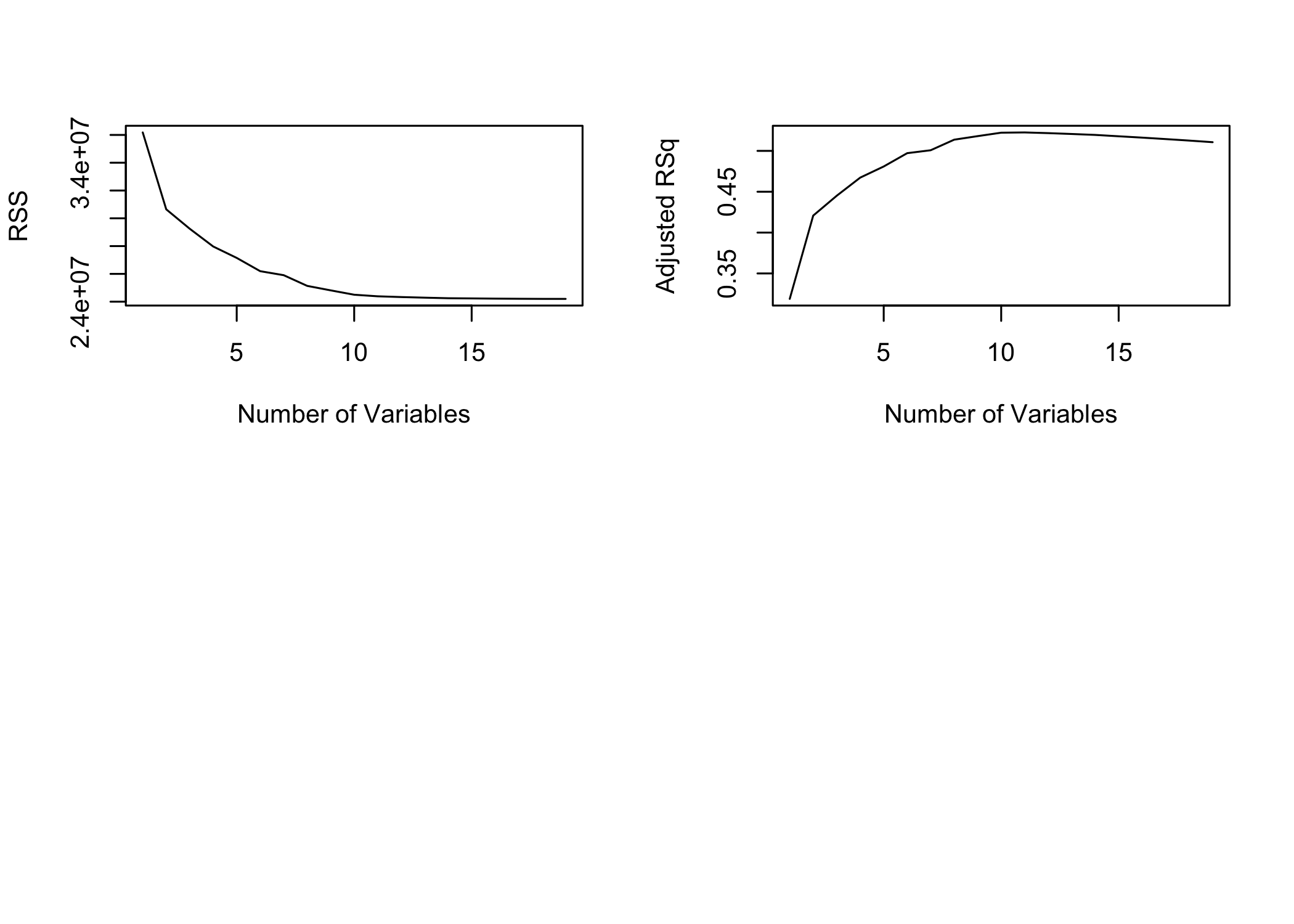

• points() adds points to an existing plot
  
• which.max() identifies the location of the maximum value
  
• Mark the model with the largest adjusted R^2

which.max(reg.summary$adjr2)

[1] 11

plot(reg.summary$adjr2, xlab = "Number of Variables",
    ylab = "Adjusted RSq", type = "l")
points(11, reg.summary$adjr2[11], col = "red", cex = 2, 
    pch = 20)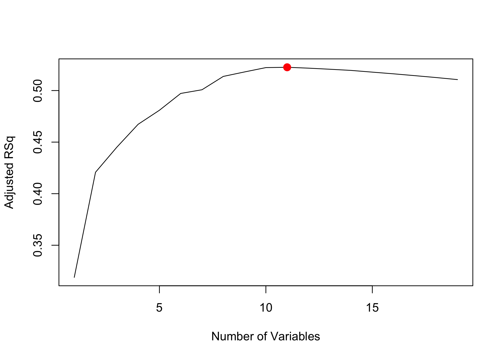

• Use which.min() to identify the best model by C_p and BIC

plot(reg.summary$cp, xlab = "Number of Variables",
    ylab = "Cp", type = "l")
which.min(reg.summary$cp)

[1] 10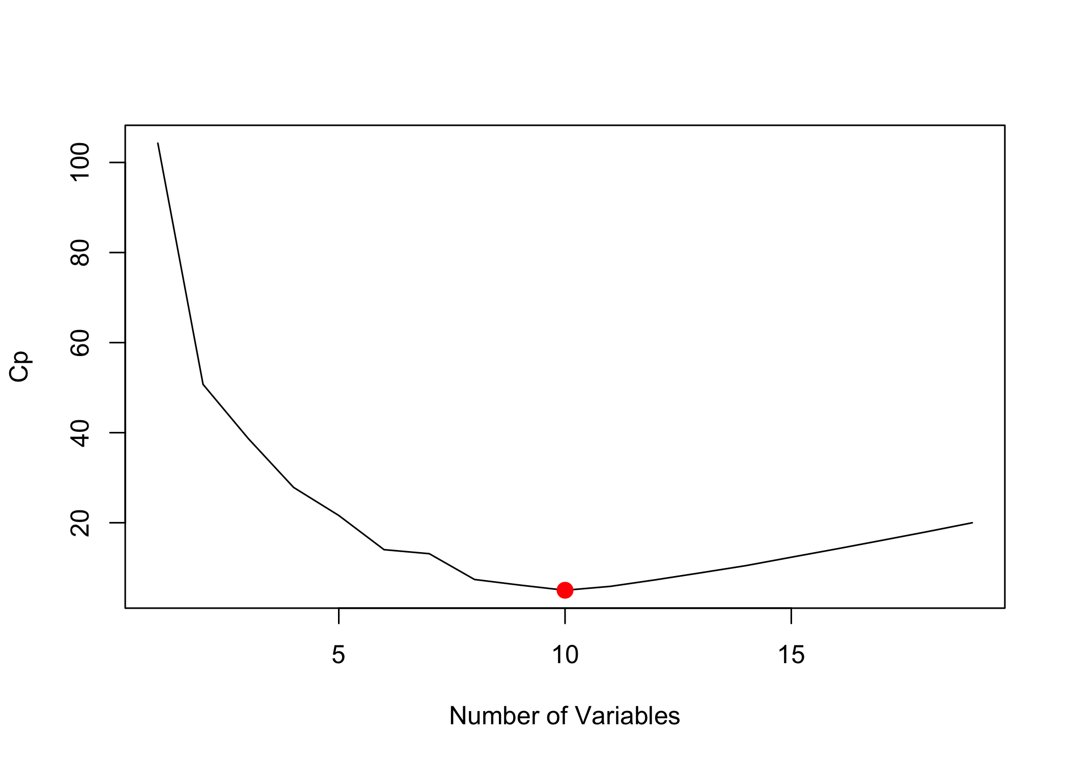

points(10, reg.summary$cp[10], col = "red", cex = 2,
    pch = 20)

which.min(reg.summary$bic)

[1] 6

plot(reg.summary$bic, xlab = "Number of Variables",
    ylab = "BIC", type = "l")
points(6, reg.summary$bic[6], col = "red", cex = 2,
    pch = 20)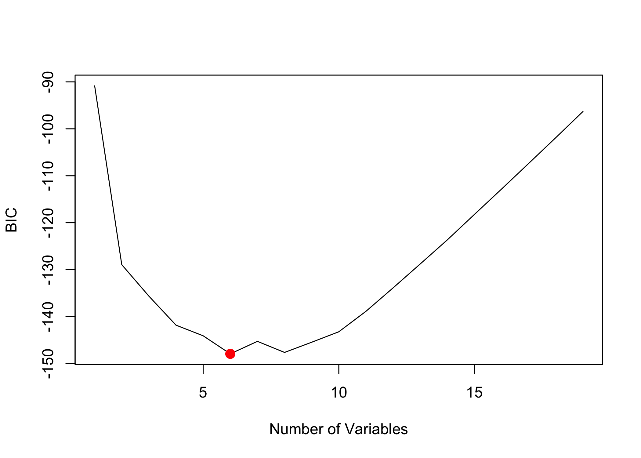

• plot.regsubsets() displays selected variables by model size
  
• Models can be ranked by:
  • r2
  • adjr2
  • Cp
  • bic

plot(regfit.full, scale = "r2")

plot(regfit.full, scale = "adjr2")

plot(regfit.full, scale = "Cp")

plot(regfit.full, scale = "bic")

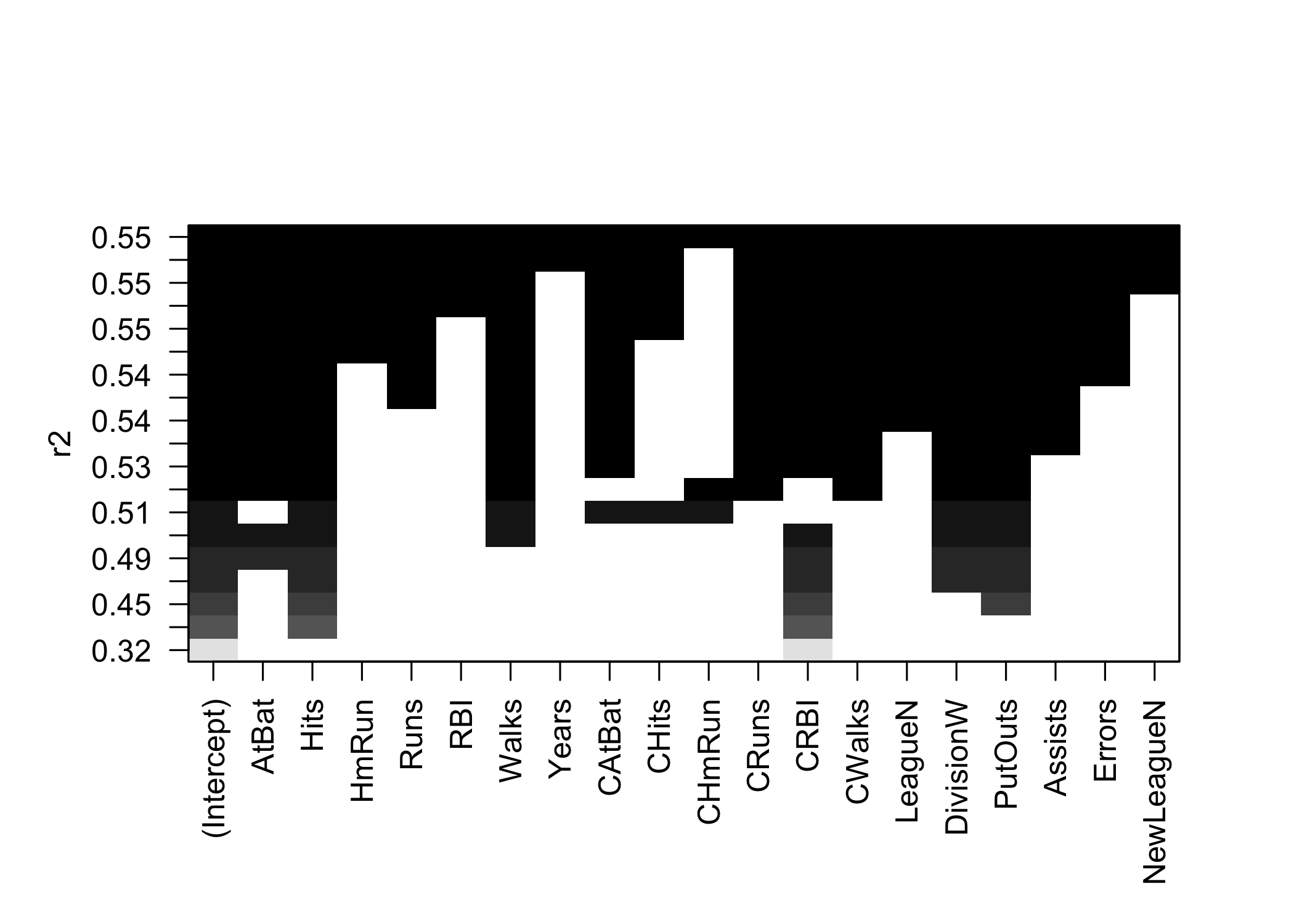
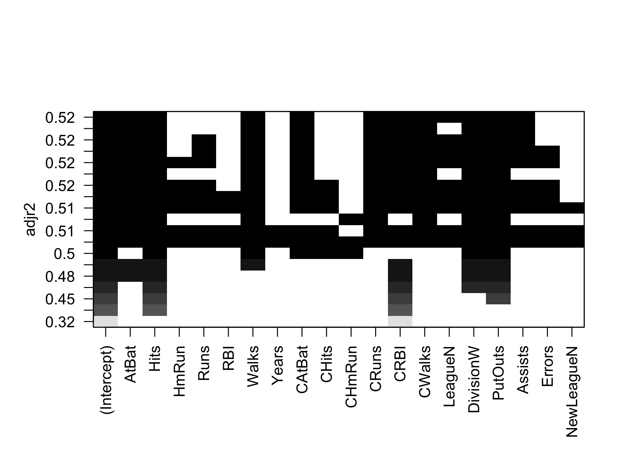
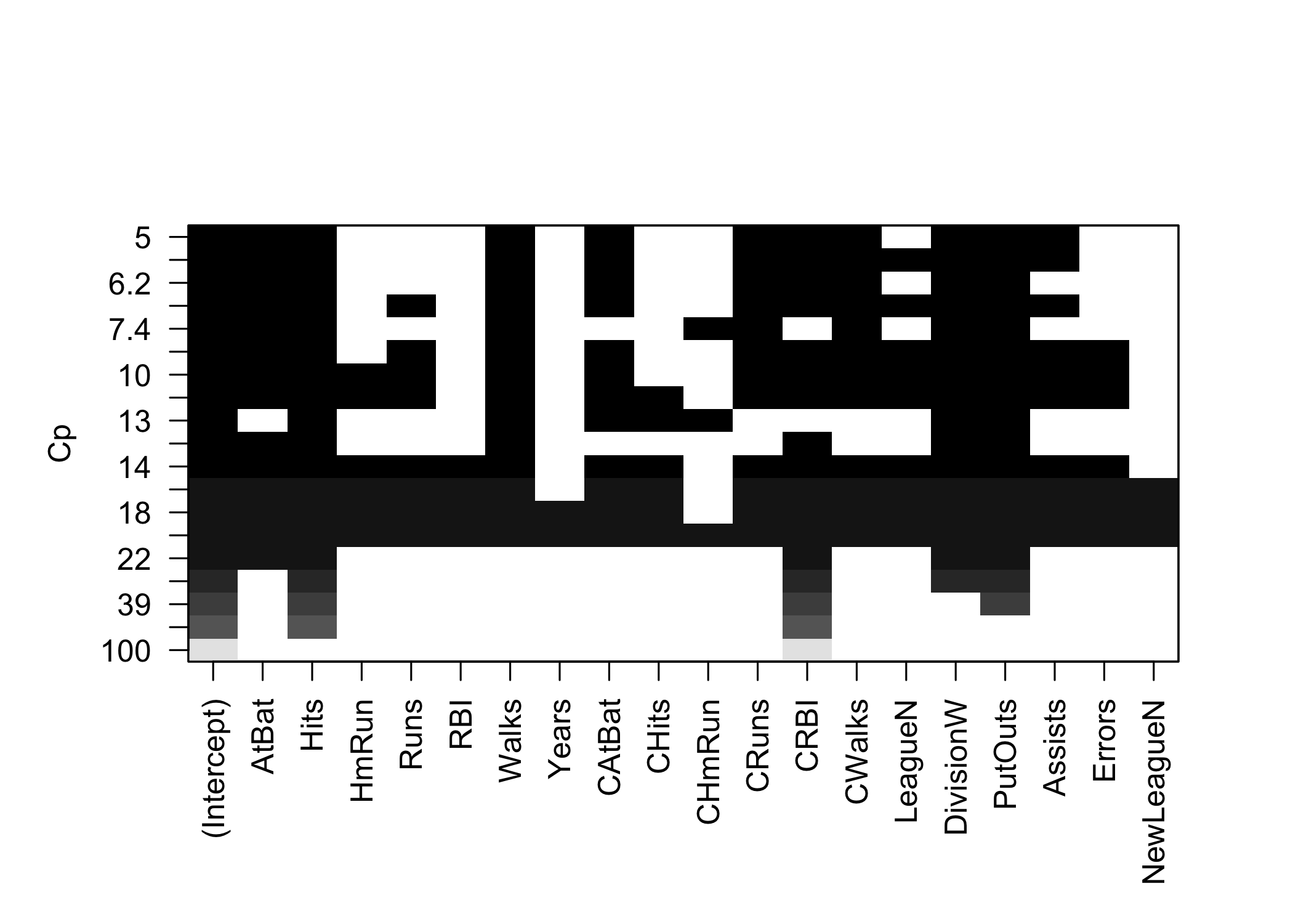
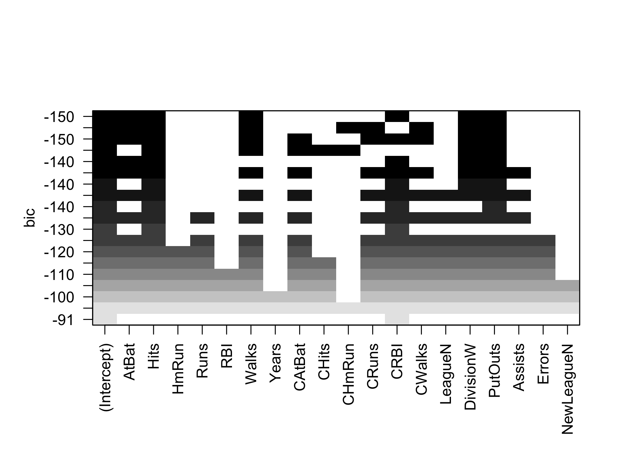
• Use coef() to inspect coefficients for a chosen model
  
• Example: the 6-variable model

coef(regfit.full, 6)

 (Intercept)        AtBat         Hits        Walks         CRBI    DivisionW 
  91.5117981   -1.8685892    7.6043976    3.6976468    0.6430169 -122.9515338 
     PutOuts 
   0.2643076 

Forward and Backward Stepwise Selection

• regsubsets() can also perform:
  • forward stepwise selection
  • backward stepwise selection
    
• Use method = "forward" or method = "backward"

regfit.fwd <- regsubsets(Salary ~ ., data = Hitters,
    nvmax = 19, method = "forward")
summary(regfit.fwd)

Subset selection object
Call: regsubsets.formula(Salary ~ ., data = Hitters, nvmax = 19, method = "forward")
19 Variables  (and intercept)
           Forced in Forced out
AtBat          FALSE      FALSE
Hits           FALSE      FALSE
HmRun          FALSE      FALSE
Runs           FALSE      FALSE
RBI            FALSE      FALSE
Walks          FALSE      FALSE
Years          FALSE      FALSE
CAtBat         FALSE      FALSE
CHits          FALSE      FALSE
CHmRun         FALSE      FALSE
CRuns          FALSE      FALSE
CRBI           FALSE      FALSE
CWalks         FALSE      FALSE
LeagueN        FALSE      FALSE
DivisionW      FALSE      FALSE
PutOuts        FALSE      FALSE
Assists        FALSE      FALSE
Errors         FALSE      FALSE
NewLeagueN     FALSE      FALSE
1 subsets of each size up to 19
Selection Algorithm: forward
          AtBat Hits HmRun Runs RBI Walks Years CAtBat CHits CHmRun CRuns CRBI
1  ( 1 )  " "   " "  " "   " "  " " " "   " "   " "    " "   " "    " "   "*" 
2  ( 1 )  " "   "*"  " "   " "  " " " "   " "   " "    " "   " "    " "   "*" 
3  ( 1 )  " "   "*"  " "   " "  " " " "   " "   " "    " "   " "    " "   "*" 
4  ( 1 )  " "   "*"  " "   " "  " " " "   " "   " "    " "   " "    " "   "*" 
5  ( 1 )  "*"   "*"  " "   " "  " " " "   " "   " "    " "   " "    " "   "*" 
6  ( 1 )  "*"   "*"  " "   " "  " " "*"   " "   " "    " "   " "    " "   "*" 
7  ( 1 )  "*"   "*"  " "   " "  " " "*"   " "   " "    " "   " "    " "   "*" 
8  ( 1 )  "*"   "*"  " "   " "  " " "*"   " "   " "    " "   " "    "*"   "*" 
9  ( 1 )  "*"   "*"  " "   " "  " " "*"   " "   "*"    " "   " "    "*"   "*" 
10  ( 1 ) "*"   "*"  " "   " "  " " "*"   " "   "*"    " "   " "    "*"   "*" 
11  ( 1 ) "*"   "*"  " "   " "  " " "*"   " "   "*"    " "   " "    "*"   "*" 
12  ( 1 ) "*"   "*"  " "   "*"  " " "*"   " "   "*"    " "   " "    "*"   "*" 
13  ( 1 ) "*"   "*"  " "   "*"  " " "*"   " "   "*"    " "   " "    "*"   "*" 
14  ( 1 ) "*"   "*"  "*"   "*"  " " "*"   " "   "*"    " "   " "    "*"   "*" 
15  ( 1 ) "*"   "*"  "*"   "*"  " " "*"   " "   "*"    "*"   " "    "*"   "*" 
16  ( 1 ) "*"   "*"  "*"   "*"  "*" "*"   " "   "*"    "*"   " "    "*"   "*" 
17  ( 1 ) "*"   "*"  "*"   "*"  "*" "*"   " "   "*"    "*"   " "    "*"   "*" 
18  ( 1 ) "*"   "*"  "*"   "*"  "*" "*"   "*"   "*"    "*"   " "    "*"   "*" 
19  ( 1 ) "*"   "*"  "*"   "*"  "*" "*"   "*"   "*"    "*"   "*"    "*"   "*" 
          CWalks LeagueN DivisionW PutOuts Assists Errors NewLeagueN
1  ( 1 )  " "    " "     " "       " "     " "     " "    " "       
2  ( 1 )  " "    " "     " "       " "     " "     " "    " "       
3  ( 1 )  " "    " "     " "       "*"     " "     " "    " "       
4  ( 1 )  " "    " "     "*"       "*"     " "     " "    " "       
5  ( 1 )  " "    " "     "*"       "*"     " "     " "    " "       
6  ( 1 )  " "    " "     "*"       "*"     " "     " "    " "       
7  ( 1 )  "*"    " "     "*"       "*"     " "     " "    " "       
8  ( 1 )  "*"    " "     "*"       "*"     " "     " "    " "       
9  ( 1 )  "*"    " "     "*"       "*"     " "     " "    " "       
10  ( 1 ) "*"    " "     "*"       "*"     "*"     " "    " "       
11  ( 1 ) "*"    "*"     "*"       "*"     "*"     " "    " "       
12  ( 1 ) "*"    "*"     "*"       "*"     "*"     " "    " "       
13  ( 1 ) "*"    "*"     "*"       "*"     "*"     "*"    " "       
14  ( 1 ) "*"    "*"     "*"       "*"     "*"     "*"    " "       
15  ( 1 ) "*"    "*"     "*"       "*"     "*"     "*"    " "       
16  ( 1 ) "*"    "*"     "*"       "*"     "*"     "*"    " "       
17  ( 1 ) "*"    "*"     "*"       "*"     "*"     "*"    "*"       
18  ( 1 ) "*"    "*"     "*"       "*"     "*"     "*"    "*"       
19  ( 1 ) "*"    "*"     "*"       "*"     "*"     "*"    "*"       

regfit.bwd <- regsubsets(Salary ~ ., data = Hitters,
    nvmax = 19, method = "backward")
summary(regfit.bwd)

Subset selection object
Call: regsubsets.formula(Salary ~ ., data = Hitters, nvmax = 19, method = "backward")
19 Variables  (and intercept)
           Forced in Forced out
AtBat          FALSE      FALSE
Hits           FALSE      FALSE
HmRun          FALSE      FALSE
Runs           FALSE      FALSE
RBI            FALSE      FALSE
Walks          FALSE      FALSE
Years          FALSE      FALSE
CAtBat         FALSE      FALSE
CHits          FALSE      FALSE
CHmRun         FALSE      FALSE
CRuns          FALSE      FALSE
CRBI           FALSE      FALSE
CWalks         FALSE      FALSE
LeagueN        FALSE      FALSE
DivisionW      FALSE      FALSE
PutOuts        FALSE      FALSE
Assists        FALSE      FALSE
Errors         FALSE      FALSE
NewLeagueN     FALSE      FALSE
1 subsets of each size up to 19
Selection Algorithm: backward
          AtBat Hits HmRun Runs RBI Walks Years CAtBat CHits CHmRun CRuns CRBI
1  ( 1 )  " "   " "  " "   " "  " " " "   " "   " "    " "   " "    "*"   " " 
2  ( 1 )  " "   "*"  " "   " "  " " " "   " "   " "    " "   " "    "*"   " " 
3  ( 1 )  " "   "*"  " "   " "  " " " "   " "   " "    " "   " "    "*"   " " 
4  ( 1 )  "*"   "*"  " "   " "  " " " "   " "   " "    " "   " "    "*"   " " 
5  ( 1 )  "*"   "*"  " "   " "  " " "*"   " "   " "    " "   " "    "*"   " " 
6  ( 1 )  "*"   "*"  " "   " "  " " "*"   " "   " "    " "   " "    "*"   " " 
7  ( 1 )  "*"   "*"  " "   " "  " " "*"   " "   " "    " "   " "    "*"   " " 
8  ( 1 )  "*"   "*"  " "   " "  " " "*"   " "   " "    " "   " "    "*"   "*" 
9  ( 1 )  "*"   "*"  " "   " "  " " "*"   " "   "*"    " "   " "    "*"   "*" 
10  ( 1 ) "*"   "*"  " "   " "  " " "*"   " "   "*"    " "   " "    "*"   "*" 
11  ( 1 ) "*"   "*"  " "   " "  " " "*"   " "   "*"    " "   " "    "*"   "*" 
12  ( 1 ) "*"   "*"  " "   "*"  " " "*"   " "   "*"    " "   " "    "*"   "*" 
13  ( 1 ) "*"   "*"  " "   "*"  " " "*"   " "   "*"    " "   " "    "*"   "*" 
14  ( 1 ) "*"   "*"  "*"   "*"  " " "*"   " "   "*"    " "   " "    "*"   "*" 
15  ( 1 ) "*"   "*"  "*"   "*"  " " "*"   " "   "*"    "*"   " "    "*"   "*" 
16  ( 1 ) "*"   "*"  "*"   "*"  "*" "*"   " "   "*"    "*"   " "    "*"   "*" 
17  ( 1 ) "*"   "*"  "*"   "*"  "*" "*"   " "   "*"    "*"   " "    "*"   "*" 
18  ( 1 ) "*"   "*"  "*"   "*"  "*" "*"   "*"   "*"    "*"   " "    "*"   "*" 
19  ( 1 ) "*"   "*"  "*"   "*"  "*" "*"   "*"   "*"    "*"   "*"    "*"   "*" 
          CWalks LeagueN DivisionW PutOuts Assists Errors NewLeagueN
1  ( 1 )  " "    " "     " "       " "     " "     " "    " "       
2  ( 1 )  " "    " "     " "       " "     " "     " "    " "       
3  ( 1 )  " "    " "     " "       "*"     " "     " "    " "       
4  ( 1 )  " "    " "     " "       "*"     " "     " "    " "       
5  ( 1 )  " "    " "     " "       "*"     " "     " "    " "       
6  ( 1 )  " "    " "     "*"       "*"     " "     " "    " "       
7  ( 1 )  "*"    " "     "*"       "*"     " "     " "    " "       
8  ( 1 )  "*"    " "     "*"       "*"     " "     " "    " "       
9  ( 1 )  "*"    " "     "*"       "*"     " "     " "    " "       
10  ( 1 ) "*"    " "     "*"       "*"     "*"     " "    " "       
11  ( 1 ) "*"    "*"     "*"       "*"     "*"     " "    " "       
12  ( 1 ) "*"    "*"     "*"       "*"     "*"     " "    " "       
13  ( 1 ) "*"    "*"     "*"       "*"     "*"     "*"    " "       
14  ( 1 ) "*"    "*"     "*"       "*"     "*"     "*"    " "       
15  ( 1 ) "*"    "*"     "*"       "*"     "*"     "*"    " "       
16  ( 1 ) "*"    "*"     "*"       "*"     "*"     "*"    " "       
17  ( 1 ) "*"    "*"     "*"       "*"     "*"     "*"    "*"       
18  ( 1 ) "*"    "*"     "*"       "*"     "*"     "*"    "*"       
19  ( 1 ) "*"    "*"     "*"       "*"     "*"     "*"    "*"       

• Best subset, forward, and backward selection may agree for small models
  
• They can differ for larger models

coef(regfit.full, 7)

 (Intercept)         Hits        Walks       CAtBat        CHits       CHmRun 
  79.4509472    1.2833513    3.2274264   -0.3752350    1.4957073    1.4420538 
   DivisionW      PutOuts 
-129.9866432    0.2366813 

coef(regfit.fwd, 7)

 (Intercept)        AtBat         Hits        Walks         CRBI       CWalks 
 109.7873062   -1.9588851    7.4498772    4.9131401    0.8537622   -0.3053070 
   DivisionW      PutOuts 
-127.1223928    0.2533404 

coef(regfit.bwd, 7)

 (Intercept)        AtBat         Hits        Walks        CRuns       CWalks 
 105.6487488   -1.9762838    6.7574914    6.0558691    1.1293095   -0.7163346 
   DivisionW      PutOuts 
-116.1692169    0.3028847 

Choosing Among Models Using the Validation-Set Approach and Cross-Validation

• Model size can also be selected using:

  • validation set
  • cross-validation

• Important: all model-fitting steps must use only the training data
  

• Variable selection must also be performed within the training set

• Create a training/test split
  

• train is TRUE for training observations
  

• test is TRUE for test observations

set.seed(1)
train <- sample(c(TRUE, FALSE), nrow(Hitters),
    replace = TRUE)
test <- (!train)

• Perform best subset selection on the training data only

regfit.best <- regsubsets(Salary ~ .,
    data = Hitters[train, ], nvmax = 19)

• Build a model matrix for the test data

test.mat <- model.matrix(Salary ~ ., data = Hitters[test, ])

• Compute validation error for each model size
  
• For each i:
  • extract coefficients
  • compute predictions
  • compute test MSE

val.errors <- rep(NA, 19)
for (i in 1:19) {
 coefi <- coef(regfit.best, id = i)
 pred <- test.mat[, names(coefi)] %*% coefi
 val.errors[i] <- mean((Hitters$Salary[test] - pred)^2)
}

• Select the model with the smallest validation error

val.errors

 [1] 164377.3 144405.5 152175.7 145198.4 137902.1 139175.7 126849.0 136191.4
 [9] 132889.6 135434.9 136963.3 140694.9 140690.9 141951.2 141508.2 142164.4
[17] 141767.4 142339.6 142238.2

which.min(val.errors)

[1] 7

coef(regfit.best, 7)

 (Intercept)        AtBat         Hits        Walks        CRuns       CWalks 
  67.1085369   -2.1462987    7.0149547    8.0716640    1.2425113   -0.8337844 
   DivisionW      PutOuts 
-118.4364998    0.2526925 

• regsubsets() has no built-in predict() method
  
• Define a custom prediction function for reuse

predict.regsubsets <- function(object, newdata, id, ...) {
  form <- as.formula(object$call[[2]])
  mat <- model.matrix(form, newdata)
  coefi <- coef(object, id = id)
  xvars <- names(coefi)
  mat[, xvars] %*% coefi
}

• Refit best subset selection on the full dataset
  
• Then extract the chosen model size from the full data

regfit.best <- regsubsets(Salary ~ ., data = Hitters,
    nvmax = 19)
coef(regfit.best, 7)

 (Intercept)         Hits        Walks       CAtBat        CHits       CHmRun 
  79.4509472    1.2833513    3.2274264   -0.3752350    1.4957073    1.4420538 
   DivisionW      PutOuts 
-129.9866432    0.2366813 

• The best 7-variable model on the full data may differ from the one on the training set

• Now use cross-validation for model selection
  

• Create:

  • 10 folds
  • a matrix to store CV errors

k <- 10
n <- nrow(Hitters)
set.seed(1)
folds <- sample(rep(1:k, length = n))
cv.errors <- matrix(NA, k, 19,
    dimnames = list(NULL, paste(1:19)))

• For each fold:
  • fit best subset selection on training folds
  • predict on the validation fold
  • store the MSE for each model size

for (j in 1:k) {
  best.fit <- regsubsets(Salary ~ .,
       data = Hitters[folds != j, ],
       nvmax = 19)
  for (i in 1:19) {
    pred <- predict(best.fit, Hitters[folds == j, ], id = i)
    cv.errors[j, i] <-
         mean((Hitters$Salary[folds == j] - pred)^2)
   }
 }

• Average CV errors across folds using apply()

mean.cv.errors <- apply(cv.errors, 2, mean)
mean.cv.errors

       1        2        3        4        5        6        7        8 
143439.8 126817.0 134214.2 131782.9 130765.6 120382.9 121443.1 114363.7 
       9       10       11       12       13       14       15       16 
115163.1 109366.0 112738.5 113616.5 115557.6 115853.3 115630.6 116050.0 
      17       18       19 
116117.0 116419.3 116299.1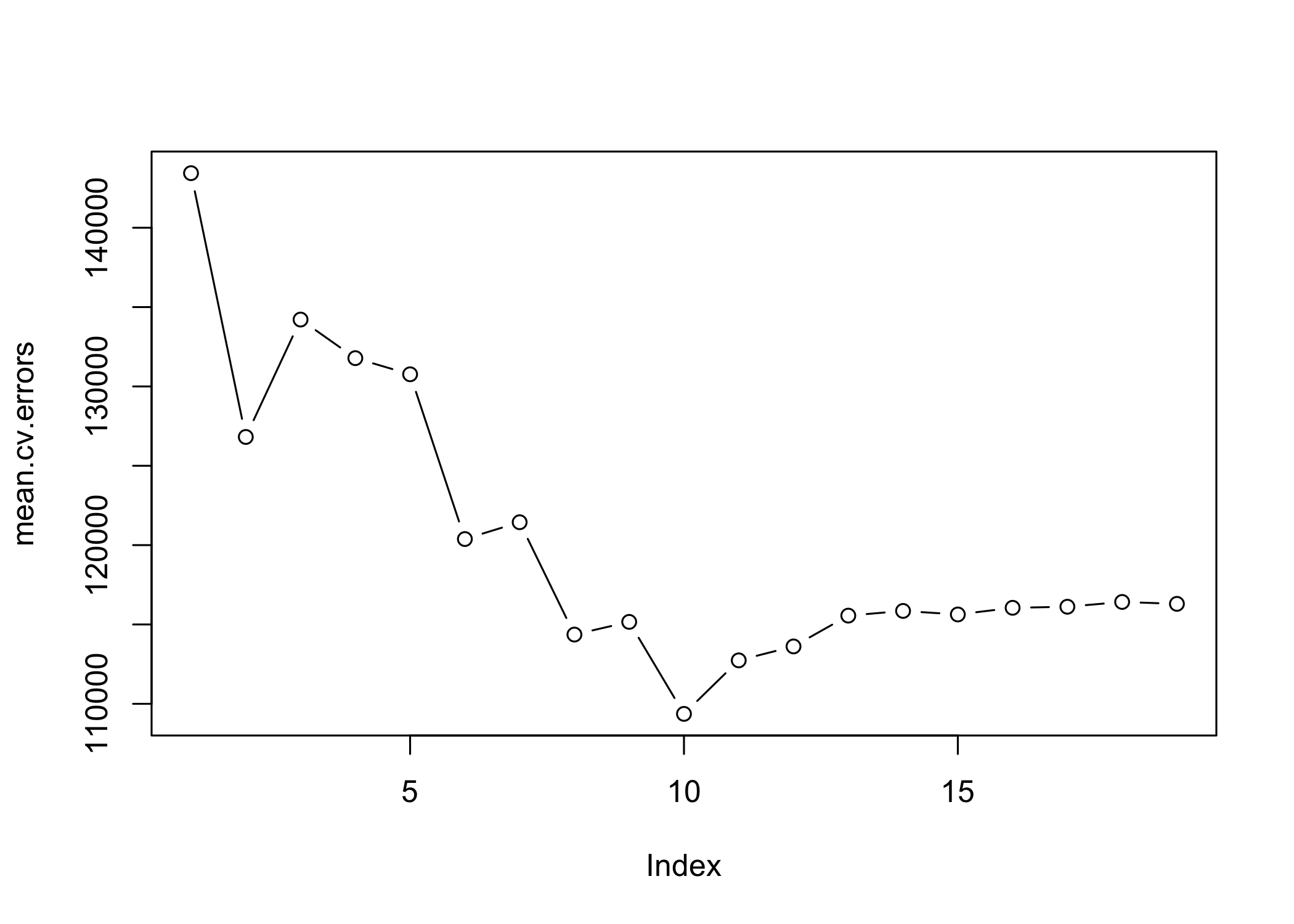 

par(mfrow = c(1, 1))
plot(mean.cv.errors, type = "b")

• Cross-validation selects the model size with minimum average CV error
  
• Refit on the full data and extract that model

reg.best <- regsubsets(Salary ~ ., data = Hitters,
    nvmax = 19)
coef(reg.best, 10)

 (Intercept)        AtBat         Hits        Walks       CAtBat        CRuns 
 162.5354420   -2.1686501    6.9180175    5.7732246   -0.1300798    1.4082490 
        CRBI       CWalks    DivisionW      PutOuts      Assists 
   0.7743122   -0.8308264 -112.3800575    0.2973726    0.2831680